PART 4

Miscellaneous

This part is the place for a variety of stuff. Some of them may grow into their own chapters or parts in the future. It also covers basic knowledge that maybe useful for those without computer science background. Lastly, there are some personal sharing from me about the life of an infrastructure architect.

Business Applications

Part 4 Chapter 1

Introduction

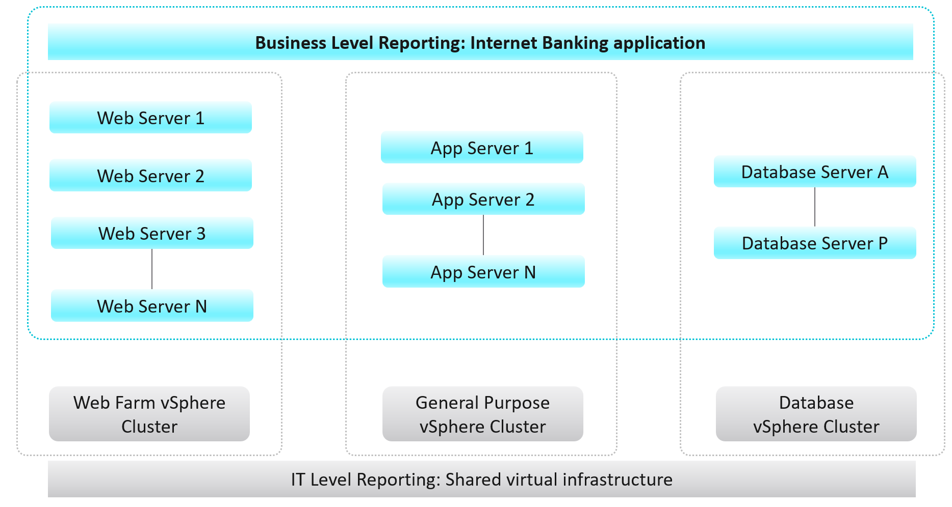
While VCF Operations maps the hierarchical infrastructure relationships out-of-the-box, there is a need for more in-depth business-oriented reporting focused on logical business constructs such as services, applications, departments, divisions, teams, groups, or any other type of logical business structure. Quantifying performance, capacity, and cost at the logical business unit level makes more relevant information to business leaders. This is because services, applications, and business units can span multiple infrastructures from private, through hybrid, to public. Not only is business-oriented reporting more intuitive for a business to consume, it also makes the IT more transparent and aligned with actual business outcomes.

Frequently, business unit stakeholders will ask IT to provide reporting around their workload’s performance, capacity, configuration, and cost. For example, a business owner may ask the following questions:

• What is the infrastructure cost for an application, service, or department?

• What can we do to reduce the infrastructure costs of our service/application?

• How much compute and storage are our application/service consuming?

• What are the poorly performing VMs in an Application Stack and why?

These questions are mostly about the underlying infrastructure, but instead of being posed at a vSphere level, they are positioned around the business applications. Traditionally, it has been very difficult for IT to answer these types of questions because typical Element Managers used by IT, represent various objects in a very rigid hierarchical fashion that does not translate well to the elastic business structure.

A different approach is necessary to address these challenges to empower business stakeholders with more accurate information. VCF Operations enables IT to analyze the underlying infrastructure and present the information in a context consumable by business decision makers.

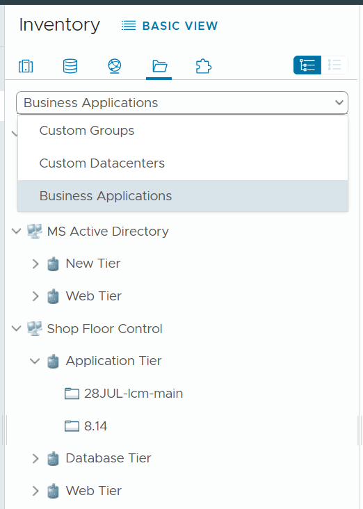
To implement the above, the first step is to design a vSphere folder structure that reflects the organisation structure. These folders and their relationships are then used by VCF Operations groups and business applications.

Implementation

| | . |

|----|----|

Business application is not an object that belongs to vSphere or VMware. It can potentially contain objects outside VMware objects. So the parent object is different. It’s called Entire Enterprise Applications, as shown on the following screenshot.

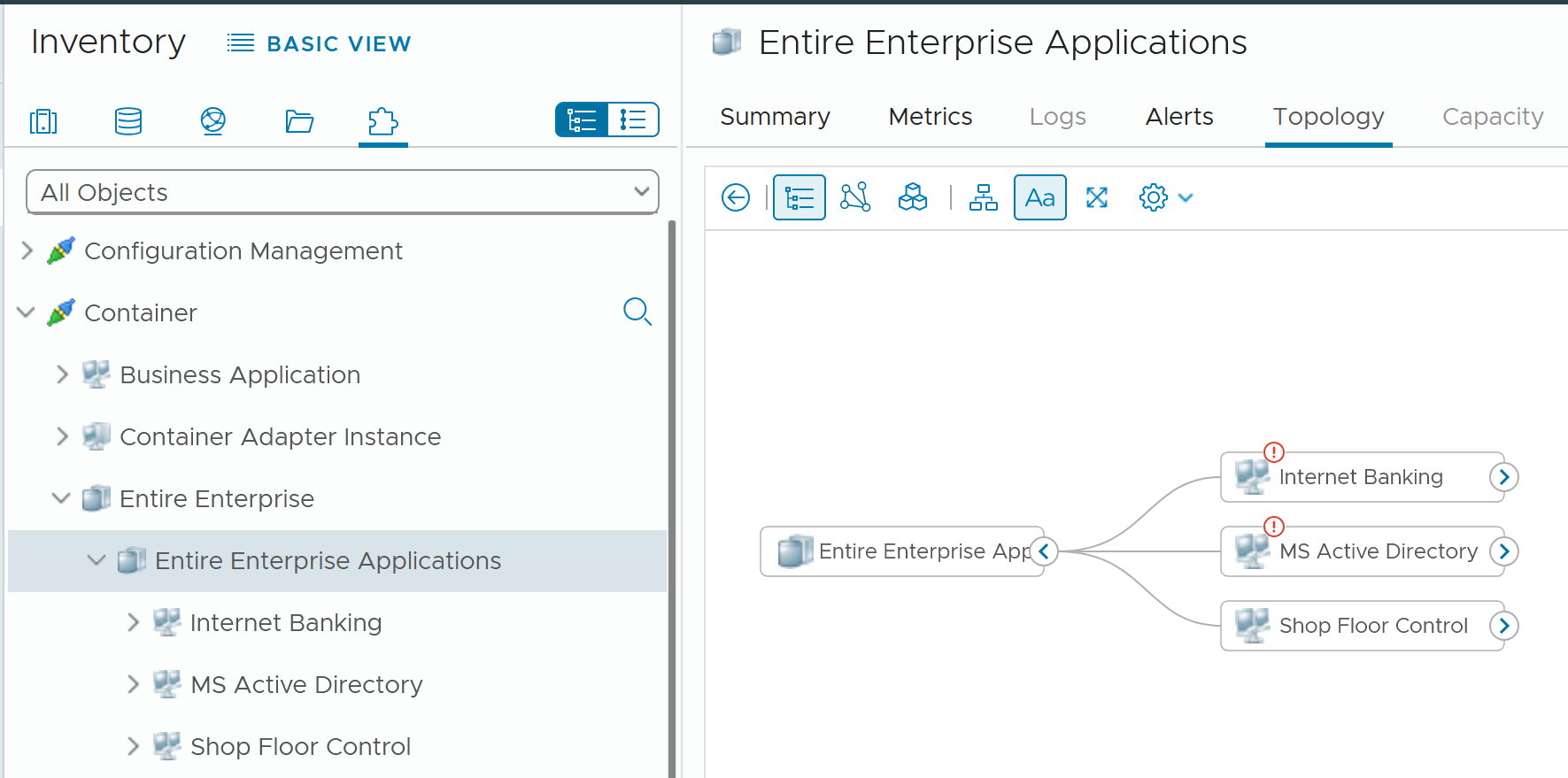
In the screenshot, you can see the structure that it’s a parent of 3 business applications

Limitation**:** The tiers are manually added. It has no dynamic membership the way Custom Groups has.

Dashboard Design

The dashboard focuses on Performance. To some extent, if the Guest OS is down, the dashboard below will detect it. If you enhance it to include availability and compliance, let me know!

The top part of the dashboard shows the overall trend.

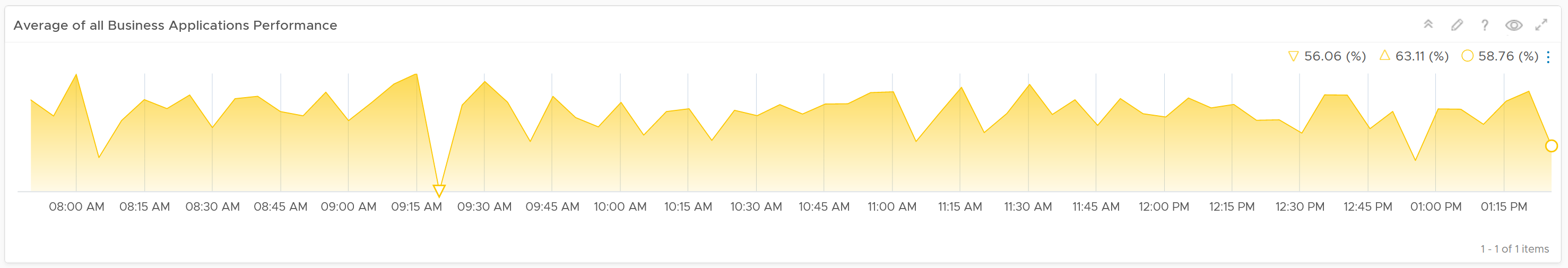
Assuming you only list your mission critical applications, you should expect the value to be good and match business reality.

The problem with average is it might mask a problem. For example, you have 2 mission critical applications. 1 has is value goes up (for whatever reason) while the other goes down. The average will fail to show it.

This is why the next row on the dashboard complements the overall picture. It has 3 columns

• The 1^st column shows all the business applications. It’s sorted by the worst performing app, judged from the most recent value.

• The 2^nd column shows the tiers within the selected business application.

• The 3^rd column shows the VMs within the tiers.

Business Applications 🡪 Tier 🡪 VM

The columns also support drill down into VM Performance dashboard and VM Capacity dashboard.

The last column, because it’s a list of virtual machines, also sports a drill down into the guest operating systems. Take note this requires Telegraf agent.

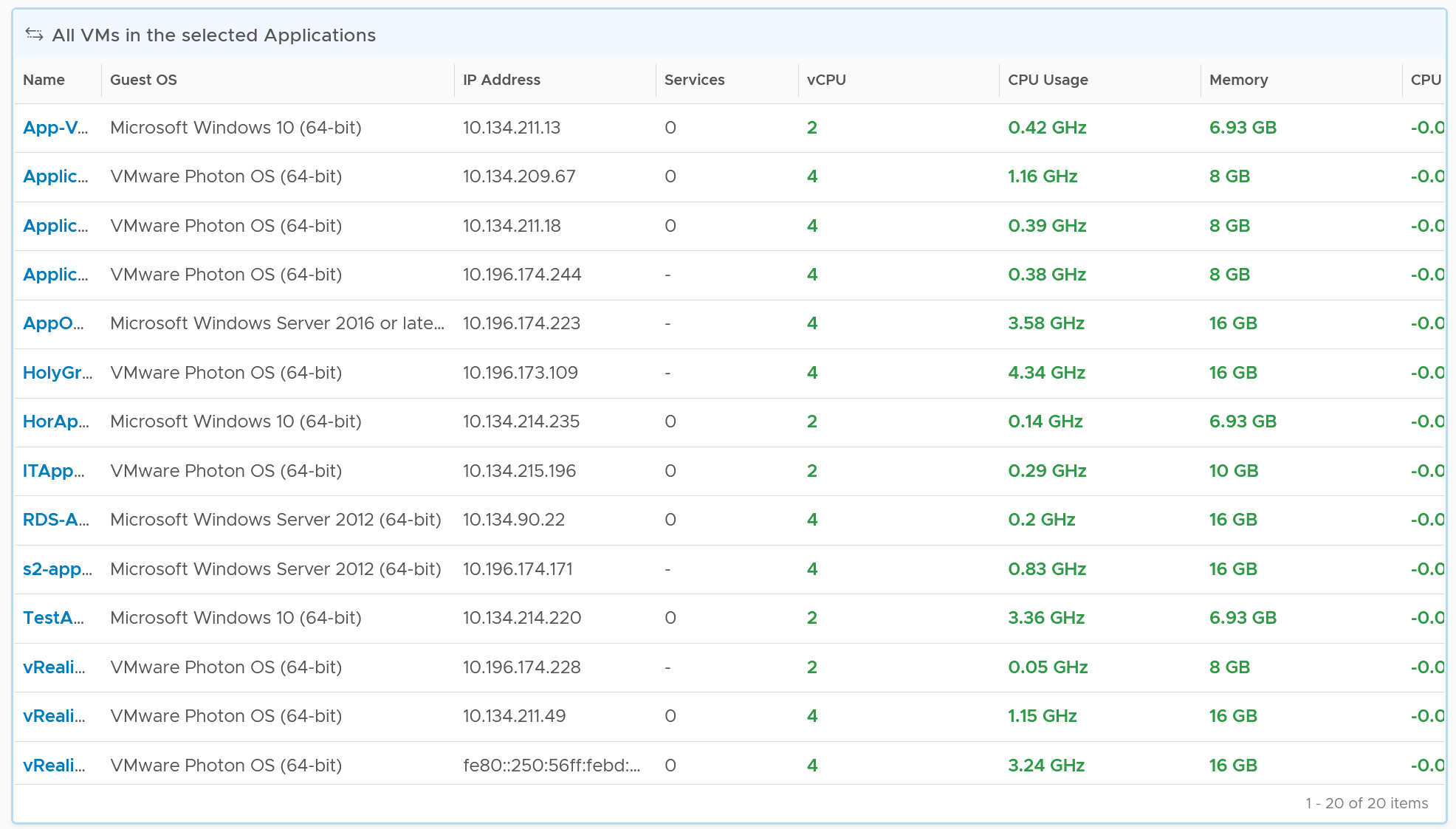
The 3 columns also drive the table underneath them. The table lists all the VMs for ease of analyzis.

Customization

You can enhance the visibility by corelation. For example, you can compare the application-level metric with infrastructure metric. CPU is a good general candidate. For example, you compare the number of web server session with the CPU Usage in GHz. If application developer releases an improved code that enable the web server to serve more users with the same resource, but the reality is the opposite, then they have something to troubleshoot.

You can enhance this by adding process-level metric. This requires you to install Telegraf agent.

A common request among VMware Admin is to give their customers a self-service access to their own VMs. The VM Owners should be given a simple portal, where they can easily see all their VMs and its performance. You can use the dashboard sharing feature of VCF Operations for a login-less access.

But what if your tenants are from different companies? They are not allowed to see one another VMs.

You don’t want to create a dashboard for each of them one by one. The challenge here is how to use the same dashboard for multiple applications teams. This requires a security mapping. Each tenant needs to have a login ID, which must be mapped to their VM.

| Role | The first step is to create a role and give it limited access. All tenants user accounts will be mapped to this role. This role should not be able to browse the inventory. Its only access is to the group of tenants. |

|----|----|

| Dashboard | Create a common dashboard and map to the role. This role can’t see any other dashboards |

| Tenant | For each tenant, you need to create a user ID. This ID is then mapped to a group. The group has the tenant VMs. In this way, the tenant ID will not be able to see other VMs. |

Capacity

In order to calculate the capacity demand, you need to know whether it is active-passive or active-active set up.

CPU Consumption =

(

If Active-Active then Average (VM Member CPU Usage) Else Max (VM Member CPU Usage)

)

/

Min (VM Member Total Capacity) * 100%

The above gives you a number in percentage, making it easier to see across many tiers. Let me know if you find a use case for absolute numbers (in GHz for CPU and GB for memory)

For total capacity, we take the lowest value among the members VM.

Part 4 Chapter 2

I’ve used the product since 1.0. When I first saw super metrics, it was one of those “is this created for me?” moments. The ability to analyze hundreds of metrics by creating my own metrics enabled me to do my job better. I was a pre-sales engineer but I spent a lot of time helping my customers troubleshooting and optimizing their environment.

Introduction

Super metrics are derived metrics that can be used to measure performance, utilization, and cost by different business units and applications, or in this case, the Custom Group into which the VMs are placed. Super metrics contain simple algebraic formulas that allow Aria Operations to measure various aspects of the Custom Groups, which contain business unit–related VMs.

At the most basic level, super metrics enable the ability to extend built-in metrics by adding new metrics that provide additional insight. This is especially important for Custom Groups as they only come with basic badge and population metrics. Having a set of more comprehensive predefined metrics is not optimal since Custom Groups can contain a mix of vastly different objects such Hosts and Datastores. For example: CPU related metrics would not be applicable to the Datastores.

This is also where the not-so-obvious power of super metrics becomes apparent. The super metrics employed to quantify Custom Groups use the concept of Relative Reference, or Depth, which allows Aria Operations to look inside of a container/bucket, measure what is in it, and return the value at the container level rather than the object being measured. This ability empowers the user to create a number of algorithms leveraging the built-in functions and collected time-series data.

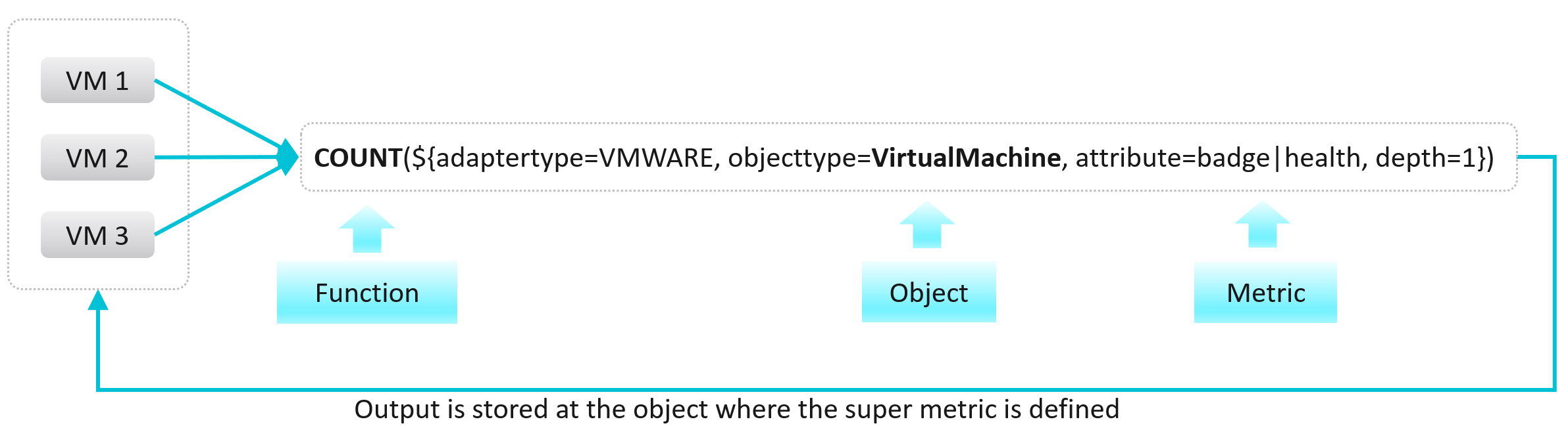
It is a programming language with mathematical formula that contains a combination of one or more metrics for one or more objects. Once you create a super metric, it persists over time and can be used for different interactions just like any other metric. It can be used in views, reports, dashboards and symptom definitions.

Super metrics are created with a list of operators and functions. These can be further combined and operated using several conditional expressions like ‘where’ or ‘if-else’.

Note that it calculates the present value. You can’t compare against historical data. That means you can’t do things such as counting the number of times an object crosses a particular threshold. You can only set the value to 1 if the threshold is crossed. To see the total over time, use the summation feature in View List.

Before starting to create a super metric, make sure you identify the following:

• Objects or object types that are involved

• Metrics which will need to be used.

• How to combine the metrics? Which operator, function or expression to use?

• Which object type will be used to assign super metric?

• Policy in which super metric will need to be enabled

Basic Functions

The maximum, minimum, average and sum functions are simple functions that can quickly summarize a large number of objects. I will provide some examples demonstrating the various features of super metrics functions and operators. More is covered in the manual.

There are also many examples in the repository of super metrics.

Example 1

Maximum CPU Ready (%) among VMs within a group of clusters providing same class of service.

max( ${ adaptertype=VMWARE, objecttype=VirtualMachine, metric=cpu|readyPct, depth=3 } )

Maximum Memory Balloon (%) among VMs within a group of clusters providing same class of service.

max( ${ adaptertype=VMWARE, objecttype=VirtualMachine, metric=mem|balloonPct, depth=3 } )

Depth=3 is used since the super metric is applied at a custom group level which is 3 levels up the VM object whose metric is used. The hierarchy is Group 🡪 Cluster 🡪 ESXi Host 🡪 VM.

Tip: If you use the same super metric for different levels, specify the deepest one.

Example 2

Sum of vCPUs provisioned on all VMs in a group of VM.

sum( ${ adaptertype=VMWARE, objecttype=VirtualMachine, metric=cpu|corecount_provisioned, depth=1 } )

Depth=1 is sufficient as the VM is directly under the group. No need to manually change the depth.

Average of CPU Usage with all VMs in a custom group:

avg( ${ adaptertype=VMWARE, objecttype=VirtualMachine, metric=cpu|usage_average, depth=3 } )

Default Value

Return CO2 Emission if the metric exists. If not, return 0.744 by default.

${this, metric=CustomProperty|CO2 Emission, defval=0.744}

The above is handy if the metric may not exist and you want to specify a default value.

‘Where’ Clause

Things get more powerful and complex once you need to specify a condition.

Use Case: Count of all VMs in the environment which has CPU usage greater than 60% at that time.

count(

${ adaptertype=VMWARE, objecttype=VirtualMachine, metric=cpu|usage_average, depth=5,

where=($value > 60)

}

)

Note: you specify 60 not 60% or 0.6. It has to match the metric value.

Use Case: Count of all Microsoft Windows VMs.

That means you need to do a string comparison. You also need to know the actual values used by the property field.

count(

${ adaptertype=VMWARE, objecttype=VirtualMachine, attribute=summary|guest|fullName, depth=5,

where="summary|guest|fullName startsWith ‘Microsoft Windows’"

}

)

Another example

sum(

${ adaptertype=VMWARE, objecttype=HostSystem, attribute=mem|host_provisioned, depth=1,

where="runtime|connectionState equals connected"

}

)

The choice for string comparison is

equals

contains

startsWith

endsWith

!equals

!contains

!startsWith

!endsWith

Use Case: Compute the percentage of VMs with CPU Ready > 1%.

That means you need to divide the number of VM against the total number of running VM.

count(

${ adaptertype=VMWARE, objecttype=VirtualMachine, metric=cpu|readyPct, depth=8, where=”>1” }

)

/

${ this, metric=summary|running_vms }

* 100

The last line in the code is to manually convert into percentage.

Use Case: Count of all VMs with CPU usage > 70% OR memory usage > 60%

This is a double comparison, with an OR clause. The formula gets complex as super metric is actually a run time code that gets executed directly. There is no translation!

count(

${ adaptertype=VMWARE, objecttype=VirtualMachine, metric=cpu|usage_average, depth=8,

where= ( $value > 70

||

${metric=mem|usage_average } > 60

)

}

)

Notice the first comparison simply uses the variable $value, because it’s actually defined in the metric=.

Use Case: Count of all VMs which are not Windows based or Redhat based.

This means you need to negate the comparison. The negation has to be done outside the two comparison.

count(

${ adaptertype=VMWARE, objecttype=VirtualMachine, metric=summary|guest|fullName, depth=5,

where= (! ($value contains 'Microsoft Windows' || $value contains 'Redhat') )

}

)

If Then Else

This takes you deeper into Java programming 😊

Use Case: Count of provisioned vCPUs and if it is equal to 4, return value “1” and if it is not equal to 4, return a value “0”.

count( ${this, metric=cpu|corecount_provisioned, depth=1, where= ($value == 4)} )

? 1

: 0

Use Case: Find the “Actual Recommended vCPU” for a VM.

While using the rightsizing feature, VCF Operations provide the vCPUs to be removed or added based on if it is an oversized or undersized VM. The following logic can be used find the actual recommended values:

If the value of Recommended vCPUs to add is 0,

then Actual Recommended vCPU = Provisioned vCPUs – Recommended vCPUs to remove (as an Oversized VM ),

else Actual Recommended vCPU = Provisioned vCPUs + Recommended vCPUs to add ( as an Undersized VM ).

${this, metric=summary|undersized|vcpus} == 0

?

( ${this, metric=cpu|corecount_provisioned} - ${this, metric=summary|oversized|vcpus} )

:

( ${this, metric=cpu|corecount_provisioned} + ${this, metric=summary|undersized|vcpus} )

This formula uses the $this, a reference to the object itself. So the context is not other object.

For completeness, let’s do the same for memory. Since the default unit is KB, we would like to convert into GB.

If the value of Recommended Memory to add  is 0,

then Actual Recommended Memory = Provisioned memory – Recommended Memory to remove (as an Oversized VM),

else Actual Recommended Memory = Provisioned Memory + Recommended Memory to add (as an Undersized VM)

(

${this, metric=summary|undersized|memory} == 0

?

( ${this, metric=mem|guest_provisioned} - ${this, metric=summary|oversized|memory} )

:

( ${this, metric=mem|guest_provisioned} + ${this, metric=summary|undersized|memory} )

)

/ 1048576

Take note there is no Case Statement. So you gotta use Nested IF as workaround.

Instanced Value

Some metrics and properties in VCF Operations exist as instance value, meaning they are repeated for each instance. The advantage of this it reduces the number of children object. The disadvantage is in visualization, as the metrics need to be accessed via the instance and not just the object.

One way to make reporting or dashboarding easier is to aggregate the values to the object. You do this via the attribute option.

The following code adds all virtual disks space of a VM.

Sum (${adaptertype=VMWARE, objecttype=VirtualMachine, attribute=virtualDisk|configuredGB, depth=5})  

Note that where clause can be done with metric only and not attribute. You can add instanced metrics but cannot apply where clause to that.

Advanced Examples

This is where you vrealize the full capability of super metric. It’s actually a programming language that gets executed as a straight line. That means it can’t loop. Think of it as a mathematical formula.

RDM Disk Capacity

How do you sum the total capacity of RDM disks in a virtual machine, since the VM typically has VMDK disk also?

In this super metric, we check the virtual disk for the property “IsRDM” and if it is true, add that disk capacity, else set the capacity value as zero. We do it for each scsciN:N, and sum all the answers.

Limitation: you need to keep adding the disks as required.

(sum

(${this, metric=virtualDisk:scsi0:0|configuredGB, where= "virtualDisk:scsi0:0|isRDM equals true"}) ?

(${this, metric=virtualDisk:scsi0:0|configuredGB}) : 0

)

+

(sum

(${this, metric=virtualDisk:scsi0:1|configuredGB, where= "virtualDisk:scsi0:1|isRDM equals true"}) ?

(${this, metric=virtualDisk:scsi0:1|configuredGB}) : 0

)

+

(sum

(${this, metric=virtualDisk:scsi0:2|configuredGB, where= "virtualDisk:scsi0:2|isRDM equals true"}) ?

(${this, metric=virtualDisk:scsi0:2|configuredGB}) : 0

)

Tools Status

Use Case: check the VM Tools running status. If it is running, return the value of OS uptime, else return the value zero.

In this example, we’re combining where clause and If Then Else.

count( ${this, metric=summary|guest|toolsRunningStatus, where= (!($value contains 'Not Running'))}) != 0

?

( ${this, metric=sys|osUptime_latest} )

:

0

Weighted KPI

Use Case: define Performance (%) of an object. The requirement is defined in the Performance Modelling section of vSphere Metrics book.

Let’s say you have the following metrics that you want to combine into a single KPI

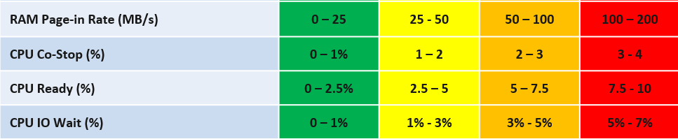
Take Other Wait for example.

• The green range is only from 0% - 1%

• That means 0% Other Wait equals to 100%, while 1% Other Wait translates into 75%.

• That means 0.8% Other Wait is 80%.

• The yellow range is 2x wider than the green range. 2% Other Wait gets translated into 62.5% as it’s in between 50% and 75%.

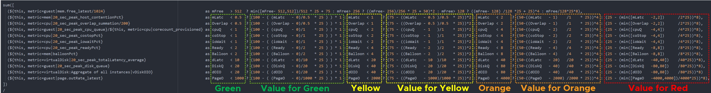
The overall code maps to the table above. The following code snippet shows the blocks for green, yellow, orange and red. No need to zoom this picture, as we will dive into the actual code line by line.

Summary

Super metric does not have a Case statement, so we have to use nested IF. The logic looks something like this

If it’s in the green range

then calculate for green range

else if it’s in the yellow range

then calculate for yellow range

else if in the orange range

then calculate for orange range

else calculate for red range

In addition to the above, you also need to assign weightage. This is critical if you have many metrics forming a KPI. for example, if there are 10 metrics, then a single red will not have enough weight to change the overall KPI red. To solve this, you assign the following weightage:

• yellow 2x the weight of green

• Orange 4x the weight of green

• Red 8x the weight of green.

Let’s see first part of the code. I’m using CPU Other Wait as the example:

(${this, metric=cpu|iowaitAvg} as ioWait < 1

? (100 - ( (ioWait - 0) / 1 * 25 ) ) * 1

: ioWait < 2

? ( 75 - ( (ioWait - 1) / 1 * 25 ) ) * 2

: ioWait < 4

? ( 50 – ( (ioWait - 2) / 2 * 25 ) ) * 4

: ( 25 – ( min([ ioWait - 4 ,4 ]) / 4 * 25 ) ) * 8

Let’s step through it.

The code “as ioWait” defines an alias. Don’t think of Alias as variable. All it does is giving a short or friendly name to a metric. They don't work for expressions.

We need to do the following translation:

| IO Wait | 0% | 1% | 2% | 4% | 8% or more |

|-----------------|:---:|:---:|:---:|:---:|:----------:|

| Translation | 100 | 75 | 50 | 25 | 0 |

The values in between need to follow the range of each bracket. Notice the width of green bracket is only 1% but the yellow is 2%. The red is special as anything above 7% needs to be capped to 0.

Using the above, let’s show a few examples of translation:

• 0.2% Other Wait 🡪 95.0

• 0.5% Other Wait 🡪 87.5

• 2.0% IO Wait 🡪 67.5

• 3.4% IO Wait 🡪 45.0

Green Range

In a perfect score, the logic will basically do 100 – 0, hence returning 100%.

In a non-perfect score, we need to prorate the value, so they land somewhere between 75 and 100.

Now let’s see how the translation is done for the Other Wait metric. The (1-0) is the range of green.

As the range is going downward, meaning the higher the IO Wait, the lower the result, it’s more intuitive to deduct from 100 than to add from 75.

If the IO Wait < 1 it performs the following

100 - ( (ioWait - 0) / (1 - 0) ) * 25

Assuming IO Wait = 0.2%, we get

100 - ( ( 0.2 - 0) / 1 ) * 25

100 - ( 0.2 ) * 25

100 - 5

You get 95, which is correct.

Yellow Range

The yellow has 2x weightage of green. So we need to multiply the final value by 2x.

( ioWait < 3 ? ( 75 - ((ioWait - 1) / (3 - 1) * 25) * 2

The line : ioWait < 3 is the ELSE branch of IF IO Wait < 1%. So we just need to check for < 3% and can safely assume it’s larger than 1%.

The (3-1) is the range of yellow. We can replace it with just the number 2 for more efficient code.

( 75 – ((ioWait - 1) / 2 * 25) ) * 2

Assuming IO Wait = 1.4%, we get

( 75 - ( (1.4 - 1) / 2 * 25) ) * 2

( 75 - ( 0.4 / 2 * 25) ) * 2

( 75 - 5 ) * 2

70 * 2

You get 140, which is correct.

The constant 50 is required to bump up the value as yellow starts at 50.

Notice you don’t need to do that funky flipping anymore 😊

Orange Range

The same logic applies for orange. The only difference is you Orange range is 50 - 25. You then multiply by 4 as it’s 4x green.

The (5-3) is the range of yellow. We can replace it with just the number 2 for more efficient code.

( 50 – ((ioWait - 3) / (5-3) * 25) ) * 4

50 - 3 – 3 / 2 * 25

50 0 / 2 * 25

50 - 0

Red Range

The red range is 5 – 7%. So 5% translates into 25%, while anything 7% or more becomes 0%.

As red is at the end of the range, we need to deal with corner case by capping any value above 7% and return 0.

The portion min([ (ioWait - 5),2 ]) caps the value to maximum 2 when IO Wait is 7% or more.

For IO Wait just above 5%, we want to return value near 2, so we get larger multiplier.

( 25 – ( min([ ioWait - 5 ,2 ]) / (7 - 5) * 25 ) ) * 8

Assuming IO Wait = 5.4%, we get

( 25 – ( min([ 5.4 - 5 ,2 ]) / 2 * 25) ) * 8

( 25 – ( min([ 0.4 ,2 ]) / 2 * 25) ) * 8

( 25 – ( 0.4 / 2 * 25) ) * 8

( 25 – 5 ) * 8

20 * 8

You get 160, which is correct.

Weightage

Can you spot a missing logic in the above?

Yes, the multiplier creates a problem. When you multiply by 2x, 4x, 8x, you need to normalize it back to the values fall within 0 – 100%.

To normalize the value back to 100%, you need to divide by the multiplier.

But how do you normalize, since each metric can have their own multiplier?

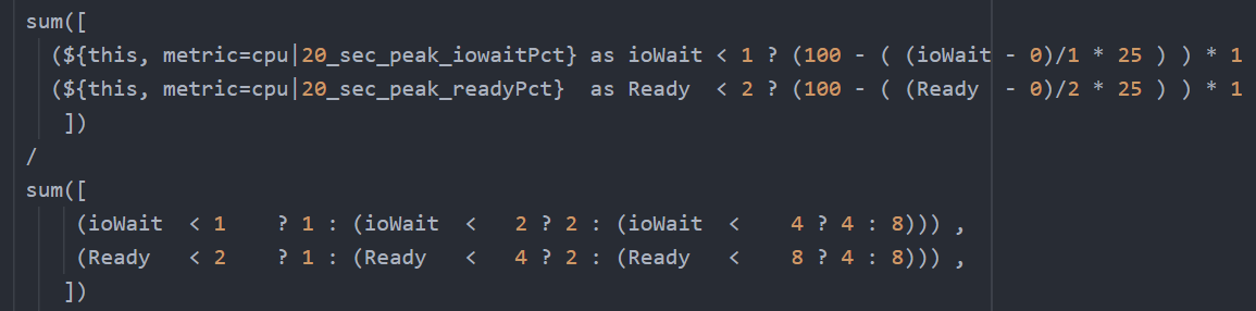
You need to have another set of nested IF statement, this time you increase the denominator correspondingly. The following shows the logic for 2 of the metrics. The multiplier is shown in red.

Sum ([

( ioWait < 1 ? 1 : ( ioWait < 2 ? 2 : ( ioWait < 4 ? 4 : 8 ) ) ) ,

( Co-stop < 1 ? 1 : ( Co-stop < 2 ? 2 : ( Co-stop < 4 ? 4 : 8 ) ) )

])

Once you have the above 2 sets, it’s a matter of dividing one over the other. The following shows part of the logic, as I want to focus on the 2 sum statements.

The complete multiplier part of the code looks like this

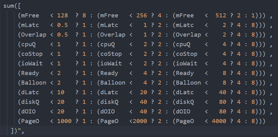
Note the entire super metric does not have error handling. If a metric does not collect, the entire super metric will return blank.

Pretty cool isn’t it? If you agree, send your thanks to Gautam Kumar and Artavazd Amirkhanyan.

VM Uptime

Use Case: calculate the VM uptime within the 5-minute collection cycle.

This particular super metric wasn’t fully implemented in the product due to the false positive from the raw vCenter counter that was discovered during validation. So I’m providing as an example of what you can do with super metric.

The up time of a VM is more complex than that of a physical machine. Just because the VM is powered on, does not mean the Guest OS is up and running. The VM could be stuck at BIOS, Windows hits BSOD or Guest OS simply hang. This means we need to check the Guest OS. If we have VMware Tools, we can check for heartbeat. But what if VMware Tools is not running or not even installed? Then we need to check for sign of life. Does the VM generate network packets, issue disk IOPS, consume RAM?

Another challenge is the frequency of reporting. If you report every 5 minutes, what if the VM was rebooted within that 5 minute, and it comes back up before the 5^th minute ends? You will miss the fact that it was down within that 5 minutes.

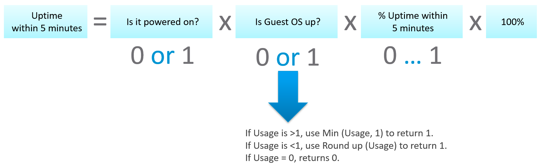
From the above, we can build a logic:

If VM Powered Off then Return 0. VM is definitely down.

Else Calculate up time within the 300 seconds period.

In the above logic, to calculate the up time, we need first to decide if the Guest OS is indeed up, since the VM is powered on.

We can deduce that Guest OS is up is it’s showing any sign of life. We can take Heartbeat from Tools. What if there no Tools or Tools not returning heartbeat? In this case, none of the metrics from Windows/Linux will be available in VCF Operations, unless we install another agent (e.g. Telegraf). We need to have fail back plan. So we check memory usage, network usage and Disk IOPS.

Can you guess why we can’t use CPU Usage?

VM does generate CPU even though it’s stuck at BIOS. We need a counter that shows 0, and not a very low number. An idle VM is up, not down.

So we need to know if the Guest OS is up or down. We are expecting binary, 1 or 0. Can you see the challenge here?

Yes, none of the metrics above is giving you binary. Disk IOPS for example, can vary from 0.01 to 10000. The “sign of life” is not coming as binary.

We need to convert them into 0 or 1. 0 is the easy part, as they will be 0 if they are down.

I’d take Network Usage as example.

• What if Network Usage is >1? We can use Min (Network Usage, 1) to return 1.

• What if Network Usage is <1? We can use Round up (Network Usage, 1) to return 1.

So we can combine the above formula to get us 0 or 1.

The last part is to account for partial up time, when the VM was rebooted within the 300 seconds sampling period. The good thing is VCF Operations tracks the OS up time every second. So every 5 minutes, the value goes up by 300 seconds. As VM normally runs >5 minutes, you end up with a very large number. Our formula becomes:

If the up time is >300 seconds then return 300 else return it as it is.

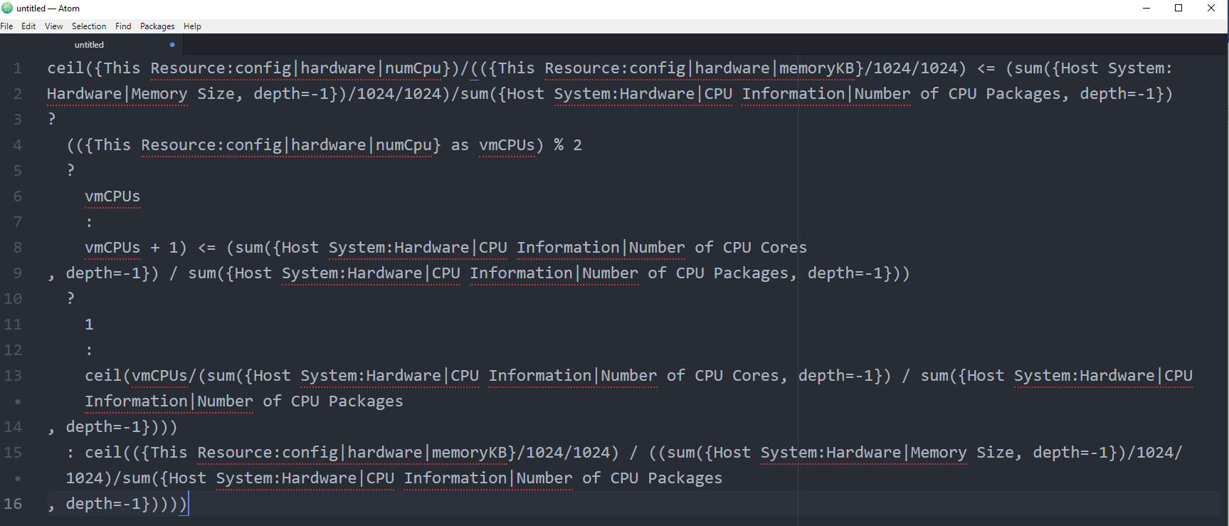
Let’s now put the formula together. Here is the logical formula:

Can you write the above formula differently? Yes, you can use If Then Else. I do not use it as it makes the formula harder to read. It’s also more resource intensive.

Let’s translate the above into a pseudocode.

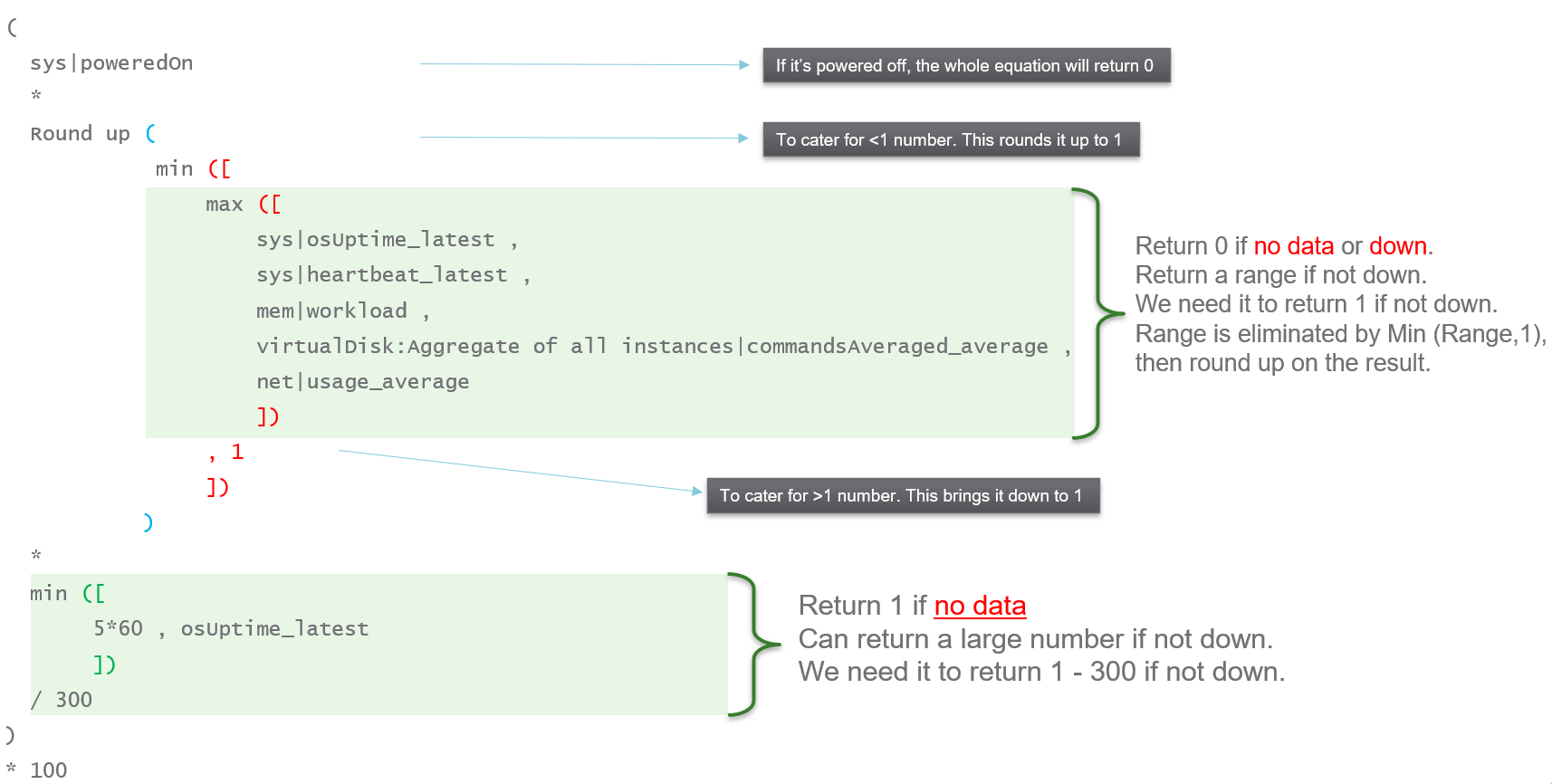
Lastly, here is what it looks like in actual code. I’ve optimized the last bit to /3. No point multiply by 100 then divide by 300.

NUMA Sizing

After VM vCPU is sized, it needs to be validated against the underlying ESXi to consider NUMA. John Diaz explains the use case here, so please read it first if you are unaware of the need for NUMA-compliant sizing.

What I’d like to highlight is John took the time to create a logical design. He visualized it on a flowchart, which I think it’s useful to ensure that the logic is bullet proof before you start coding.

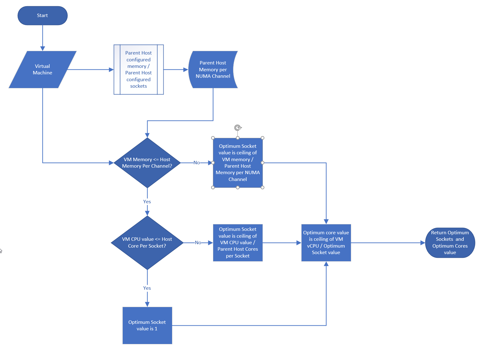
John also uses a code editor to help check the syntax. I myself have applied the same technique for long super metric.