Capacity Management

Part 1 Chapter 3

Overview

“Good” Advice

Let’s begin with this as I keep seeing it in VMware-based environment. The scope of the advice is about a VMware vSphere Cluster, but the principle applies to others such as Kubernetes, VDI or AI.

Can you figure out why the following statements are wrong? They are all well-meaning advice on the topic of Capacity Management. We’re sure you have heard them, or even given them.

Regarding vSphere Cluster RAM:

• We recommend 1:2 overcommit ratio between physical RAM and virtual RAM. Going above this is risky.

• Memory Usage on most of your clusters is high, around 90%. You should aim for 80% as you need to consider HA.

• Memory Active should not exceed 50-60%. You need a buffer between Active Memory and Consumed Memory.

• Memory should be running at high state on each host.

Regarding vSphere Cluster CPU:

• CPU Ratio on cluster “XYZ” is high at 1:5, because it is an important cluster.

• The rest of all your clusters’ overcommit ratio looks good as they are around 1:3. This gives you some buffer for spikes and HA.

• Keep the overcommit ratio to 1:4 for Tier 3 workload as they are not mission critical.

• CPU usage is around 70% on cluster “ABC”. Since they are UAT servers, don’t worry. You should get worried only when they reach 85%.

• The rest of your cluster’s CPU utilization is around 25%. This is good! You have plenty of capacity left.

Can you figure out where the mistakes are?

The mistake is they are simplified. Capacity may appear simple:

• Can you architect a cluster where the performance matches physical?\

  Easy, just don’t overcommit, or put 100% reservation for that VM.

• Can you architect a cluster that can handle monster VMs?\

  Easy, just get lots of cores per socket.\

  Easy, just get lots of core in the box.

• Can you architect with very high availability?\

  Easy, just have more HA hosts, more vSAN FTT with failure domains spread across different racks, more NSX Edges.

• Can you architect a cluster that can run lots of VMs?\

  Easy, just get lots of big hosts.

• Can you optimize the performance?\

  Sure, follow performance best practices and configure for performance. Just be prepared to pay.

• Can you squeeze the cost?\

  Sure, minimize the hardware and software cost, and choose the best bang for the buck. You know all the vendors and their technology. You know the pro and cons of each.

But how to put all the above together that optimize cost, performance, security and availabiity?

Concept

Balancing demand and supply require you to look at these 6 components below. Steps 1 and 2 are done together, and the remaining 4 steps can be done in parallel.

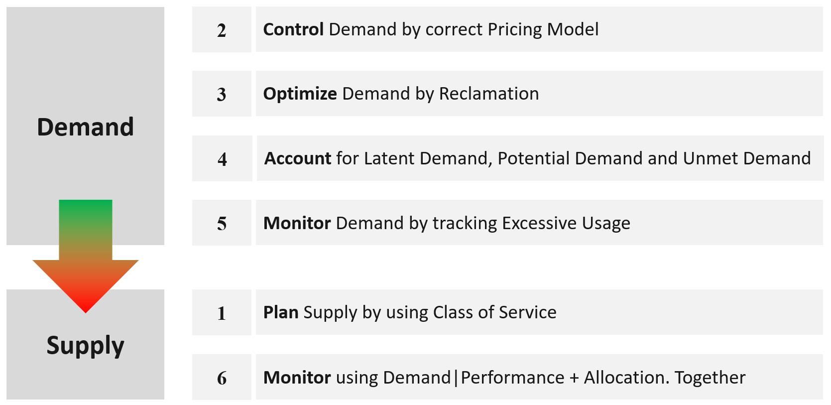
The above is less harder to do if you do it right from the start, which is why we need to begin at the planning phase.

If you start from Step 6 and ignore Step 1 and 2, you will play the lead role in a Mission Impossible movie, because you can end up with many over-provisioned VM issue. These VMs are typically the larger ones, and more important to the business. It is hard to solve this in production environment as it will involve downtime and the burden is on you to prove it will not have performance impact. Politically, it may make the team who sized the VM and justified the cost look bad.

Your best bet is to prevent the problem from happening in the first place.

VM impacts capacity in 2 ways:

• Rightsizing

• Reclamation.

Private Cloud Capacity

Your IaaS consists of 3 large components

• Compute

• Storage

• Network

Compute	It covers ESXi, cluster, resource pool, and physical server. It gets the most attention as the consumer (VM or Pod) runs in a cluster of ESXi host. It’s a good starting point, especially if you have 1:1 relationship between compute and storage.
Storage	It covers datastore, datastore cluster, vSAN, RDM, physical array, back up infrastructure, etc. It needs to be managed equally well, if you have many to many relationships between cluster and datastore. If you use vSAN HCI Mesh, then you also need to manage the storage portion carefully.
	Storage Capacity differs to Compute Capacity and presents a challenge on its own. Unlike compute capacity, which is basically vSphere cluster, storage varies in shape. The two major ones are datastore and vSAN, as local datastore and RDM are rarely used. In addition, storage has thin provisioning at both virtualization layer and physical layer. We will discuss vSAN capacity separately as it has its own unique factors such as FTT, plus it needs to consider compute too.
Network	It covers virtual and physical. It also includes switch, router, firewall, load balancer, etc. It is typically less of an issue for VMware Architect, as it’s typically done by the Network Architect. In addition, it’s common for ESXi to sport 50 Gb of bandwidth. So unless you run high bandwidth applications, such as networking VMs and web servers, running on the same ESXi hosts, you may not hit the limit.

Stages

Capacity Management requires an end-to-end plan, typically spanning multiple years, not months. Why?

There are 2 reasons:

• At the provider, the physical layers form a constraint. A rack, top of rack switch, cabling, cooling all have limits.

• At the consumer level, production workload tends to live for several years, and they change along the way.

Such a long plan requires adjustment along the way, because at the end of the day it is about comparing the reality you face with the plan you set. Good or bad is relative to your plan. If you plan for no overcommit because performance is absolute and budget is not an issue, then you’ll never run out of capacity. In other cases, that could be considered bad as you could end up with a lot of wastage.

There are 4 phases of capacity management:

Plan	Within this phase, you perform sizing and estimate how long the infrastructure will last. Depending on the project, you may even size a multi-year capacity up front. The longer the plan, the bigger the margin you need to allocate. Higher margin or buffer certainly increases the risk of excess capacity. As not all plans are confirmed, you may run multiple What If scenarios. This is the phase where you buy hardware.
Monitor	This phase starts after deployment. You begin tracking and compare the reality against plan. For example, you expect the capacity for your new DaaS project to last for 1 year. 3 months into deployment, you have 25% of your users consuming the DaaS. However, your overall utilization is already at 70%. This is a red warning, indicating your plan is off by significant margin.
Optimize	You optimize both the supply and the demand. To optimize supply, you typically perform a tech refresh. Newer hardware can bring 2x the capacity at the same cost. To optimize demand, you perform reclamation and rightsizing.
Upgrade	As the hardware reaches end of life, you either upgrade or migrate. The workload likely need vMotion somewhere else. This typically involves technology version refresh and design changes.

Capacity Management becomes easier if you begin at the planning stage. This is where you define your offering, setting the price and performance expectation. Without expectation being quantified as metrics, your customers will demand high performance as you’ve promised them “good” performance.

e first place, by using progressive pricing. This is covered in the Cost and Price Management chapter.

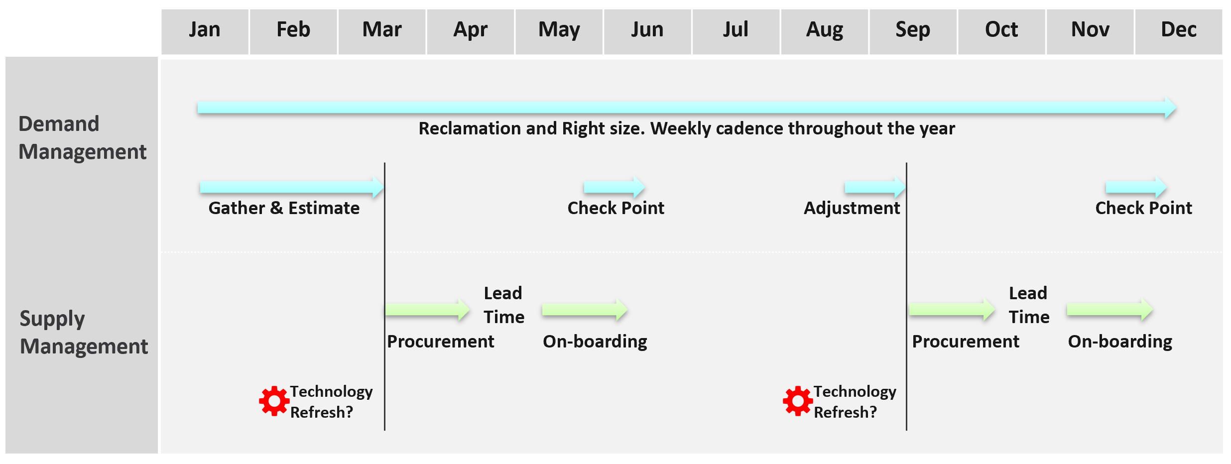
Discipline in capacity optimization is necessary due to excess wastage. Establish a weekly cadence that is executed regularly (depending on the size of the environment).

In large environment, set up upgrade cadence. Let’s take an example:

• You have 1200 ESXi hosts. Hardware depreciation and warranty is 5 years, so you replace after 5 years. That means you replace 240 hosts per year. If you do a monthly cadence, you replace ~20 servers per month.

• To balance between keeping variations low and harnessing new technology, you set the standard per year. Technology Refresh is an integral part, as new technology delivers both lower cost and higher capacity, not to mention faster performance and tighter security.

The Planning Stage

Capacity management begins long before hardware is deployed. It begins with a business plan, which decides on what class of service will be provided to serve which locations. Class of Service was covered earlier in SLA. You should also read the Performance SLA portion here, as it’s required when you overcommit the capacity.

Input	Consideration
Location	The physical location, which could be data sovereignty or network latency requirements.
Cost	It impacts the architecture and location.
Class of Service	It’s related to the type of service. In addition to IaaS, you may have VDI, Database as a Service, K8 as a service, etc.
Security	It might require traditional physical or air gap separation.
Availability	This includes HA and DR.
	Depending on the business policy, you may have to comply with Business Continuity Policy or security policy. Examples: Define the blast radius to contain major outage. This may translate that you do not design a large cluster containing large amount of VMs, as a cluster may unintentionally go down. Define the concentration risk. The number of mission critical VMs in the same datastore is capped below 250 VMs. Contain the security risk. Internet-facing VM and internal-facing VM do not share the same network.
Environment	Other than production, you may need to provide test, development, staging environments.
	What if an application needs to do a scalability test? A revenue-generating application going live may need to simulate their full load to ensure it can meet the sales demand. This scalability test can’t be performed in production environment. One solution is to triple purpose the DR cluster. It’s DR + Dev + Test, where test includes scalability test. This means the cluster size needs to be larger. If this is not possible, then burst to cloud, as it’s temporary workload.

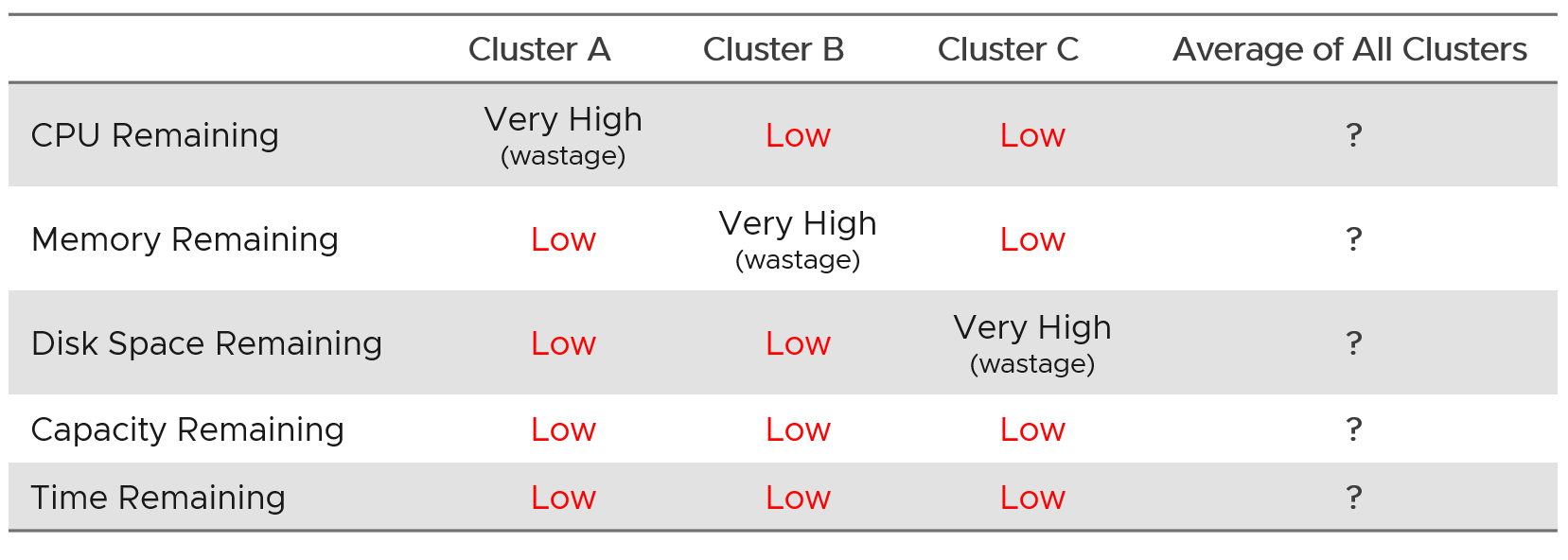
Group your operations by clusters or group of clusters. Take note that the vCenter Data Center object for example. It can contain clusters of different purposes. It will not make sense to combine the metrics into a single data center capacity remaining (%) metric, if the member clusters are not interchangeable.

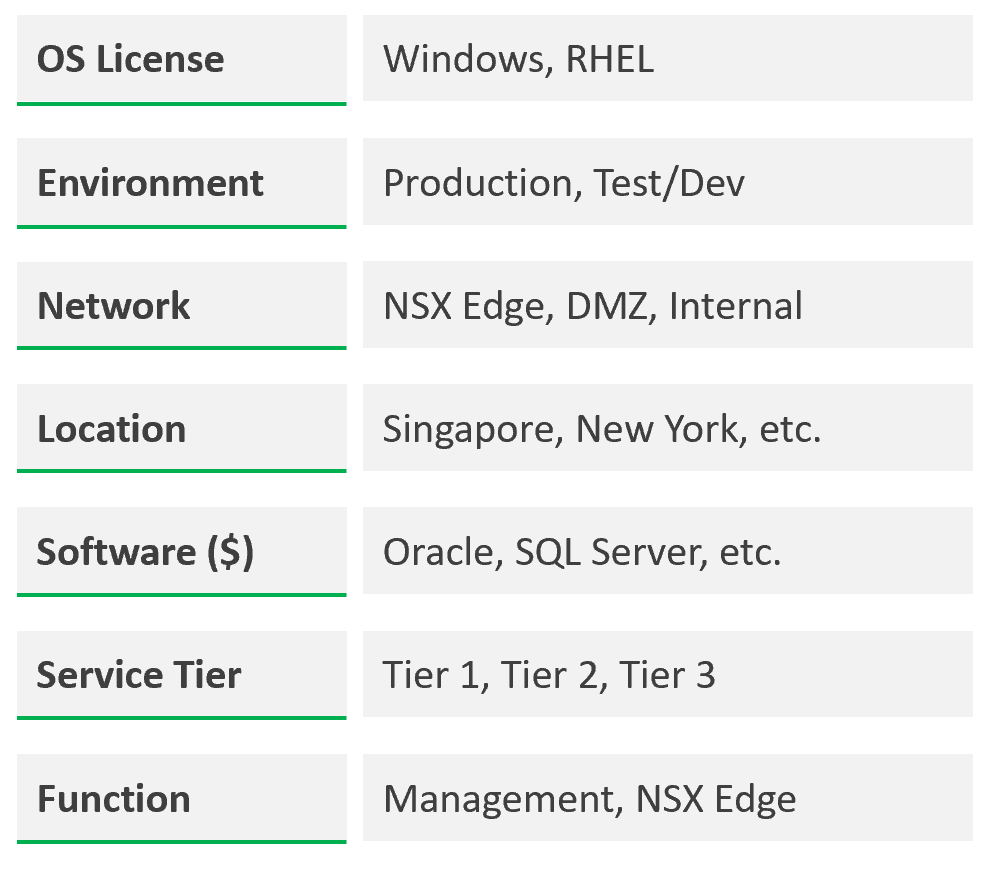
Architecture Plan

As you can see, it’s complex to balance all the above. To make it worse, what worked last year for you may not work next year as many factors change. Regardless, make an overall plan that lists all the input you need. In a large environment, list all the input considerations for vSphere Clusters.

From a capacity monitoring point of view, vSphere cluster is the smallest logical building block, due to HA + DRS + DPM. So it is correct to assume that we do capacity planning at Cluster level, and not at Host level or Data Center level.

DR solution such as Site Recovery Manager impacts capacity as you need to consider both the DR test and actual DR.

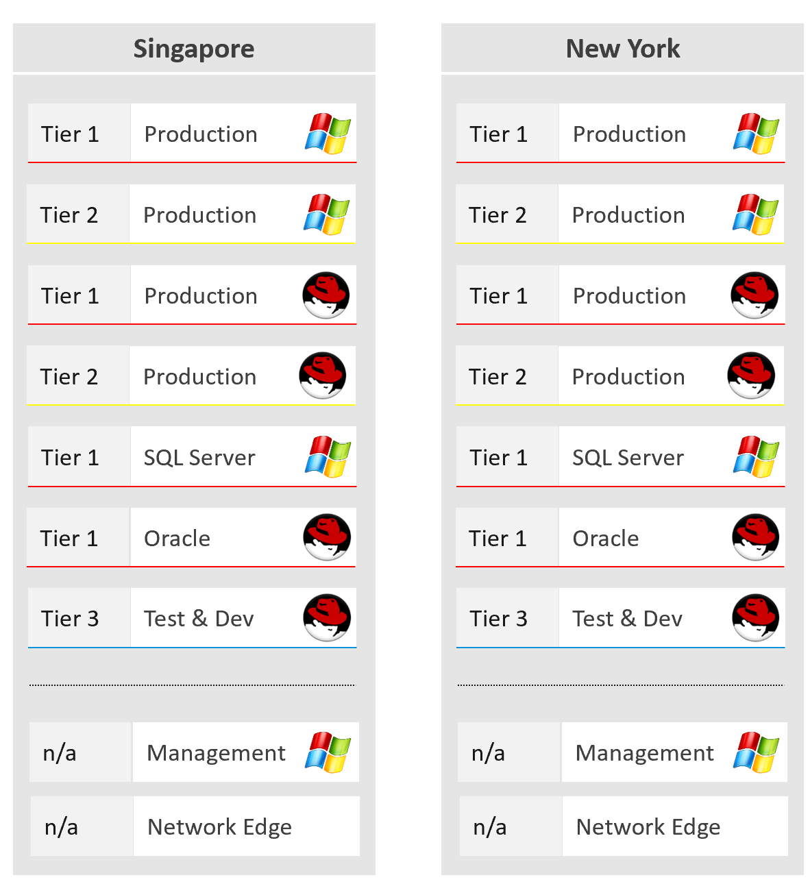
Example

The following shows a VCF environment with just 2 physical locations but 18 unique clusters. It has 7 clusters for business workloads and 2 clusters for non-business loads (overhead).

Optimized Capacity

Optimized Capacity means you fully consume what you bought, without wastage or compromising performance.

There are two areas where you can optimize:

• Consumer

• Provider

Consumer

In the consumer layer (process, guest OS, container, VM), optimize the following:

CPU	Use CPU Run Queue as primary counter, as utilization should be 100% to minimize ping pong and NUMA. Make sure all the CPU is used well by check the CPU Usage Disparity metric, as some applications tend to gravitate towards the first 8 vCPU.
Memory	Utilization should be near 100% as it contains cache (majority of pages not active). Check page fault to see if there are excessive page fault.
Disk	Rightsize the filesystem. Note this requires Windows or Linux partition modification. Reduce the usage of RDM. If you do, and you use thin provisioning at array level, check for wastage using unmap.
VM	Imbalance cluster with low ESXi utilization can be caused by monster VM. Can the applications scale horizontally instead?
Container	Do you use 1 container per VM or multiple containers per VM? If it’s >1, how do you ensure one does not dominate the others, since their size is not capped. If you use 1:1, how do you prevent container sprawl?

Provider

In the provider layer (ESXi, cluster, datastore & datastore cluster, distributed switch and port group, hardware), you can optimize the following:

Compute	Reduce pockets of resources by using larger cluster, removing Host/VM Affinity and setting DRS to be fully automated. Avoid usage of Resource Pool. Increase supply while keeping cost the same by doing a technology refresh. Avoid usage of CPU pinning. Reduce reservation. VMs in the same cluster should have same priority
Storage	Use larger datastore to minimize island of buffers. Use local datastores for agent VM or applications that do not need HA. Reduce islands of datastores by consolidating datastores that are lowly utilized.
Network	Use larger physical pipe. For example 2x 100 Gb instead of 4x 10 Gb. Use load-based teaming. Remove unused network. While network is good for segregation, VXLAN or VLAN sprawl make both management and security harder.

Capacity Model

Capacity is only possible if we can model it. That means defining the different types of capacity dimension. For each dimension, we need to define the formula for total capacity, usable capacity and consumption metrics.

4 Inputs to Capacity

Manage capacity by considering the 4 types of input below.

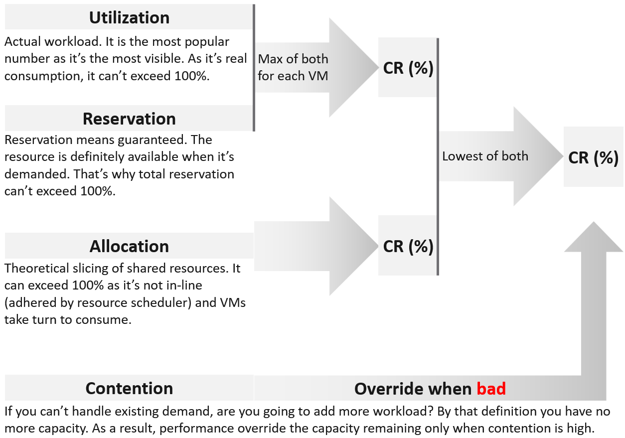
Use Reservation and Allocation to prevent utilization from going too high, and hence causing performance problem. Reservation is a stronger tool, as the kernel, DRS and HA honor it. So use it more carefully than Allocation.

Utilization and Reservation are in-line. Allocation is not.

• Because they are in-line, they cannot exceed 100%. Unlike utiilzation, reservation only kicks in when it is needed.

• Not in-line means ESXi and vCenter do not use allocation for actual resource scheduling. As a result, you can overcommit in allocation.

There are 2 levels of load:

Overcommit	To prevent utilization from going to high, you are driven by contention. If it’s high, you stop adding new load regardless of utilization
	In mixed class, use reservation to prevent overcommit from going too high. This in turn will prevent utilization from hitting 100%
Not Overcommit	This happens in mission critical where the business value of the workload far exceeds the cost of infrastructure.
	The ratio between consumer and producer is 1:1. Both utilization and contention become irrelevant as each VM can get what it wants. Allocation is the only useful input.
	Reservation does not consider hyperthreading as it’s technically hard to determine the actual CPU cycles. For CPU, each thread in a hyperthreading only gets 62.5%. So the maximum reservation is 62.5%.

Allocation is the metric you use when selling the capacity to your consumers. If you charge half price relative to full price, then your overcommit should not exceed 2:1.

Use Allocation when you want to protect the shared infrastructure from sudden spike.

The ideal scenario is the cluster is running at 100% utilization but 0% contention, because it’s working as productively as possible. You get your investment well used. This is why performance is an override, but only used when it’s bad.

Why is reclamation not included?

Because it only changes the capacity remaining (%) value when you reclaim the actual wastage.

However, wastage should be part of your SOP. It can impact your decision as wastage is prevalent. Capacity can be low, but if you can reclaim a sizeable chunk of wastage, you can defer hardware purchase.

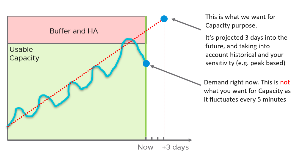
Projection

At the heart of capacity is projecting the historical consumption into the future.

The following diagram shows why projection is superior to a simple percentile calculation.

The accuracy of the prediction depends on the amount of data and the length of the cycle. If the data is limited and the pattern that matches your business cycles has not developed, the projection would not meet your expectations.

A workload with quarter end peak will naturally need at least 6 months for it to be accurate. If there is enough data, VCF Operations will consider 6+ months’ worth of data. While it gives extra weight to recent data, if there is a sudden but short-lasting change, it may not be enough to impact the projection.

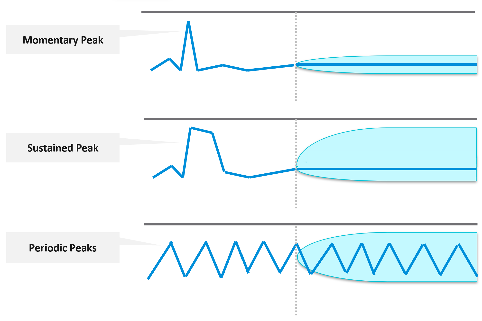
Momentary peaks that are short lived and one-off should not impact capacity planning so the impact may not be noticeable in the projection.

Sustained peaks last for a longer time and do impact projections. If the peak is not periodic, the impact on the projection lessens over time due to exponential decay. Data is exponentially weighted based on how far back in time they are, giving recent data points more important than older ones.

Periodic peaks exhibit cyclical patterns or waves, such as hourly, daily, weekly, and last day of the month. There can be multiple overlapping cyclical patterns, which will also be detected. While you should not make capacity decision based on just a few days of data, you do need the 5-minute granularity as input. A 5-minute peak that gets repeated every hour should be considered.

Exponential decay is important as newer data is more relevant, but it might make the projection visually odd. The following projection looks “make sense”, because your eyes see the whole period and give equal weightage to all data points.

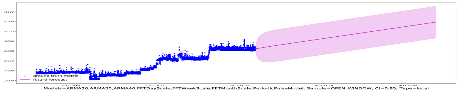
If you give higher weightage to newer data, it can potentially look like this.

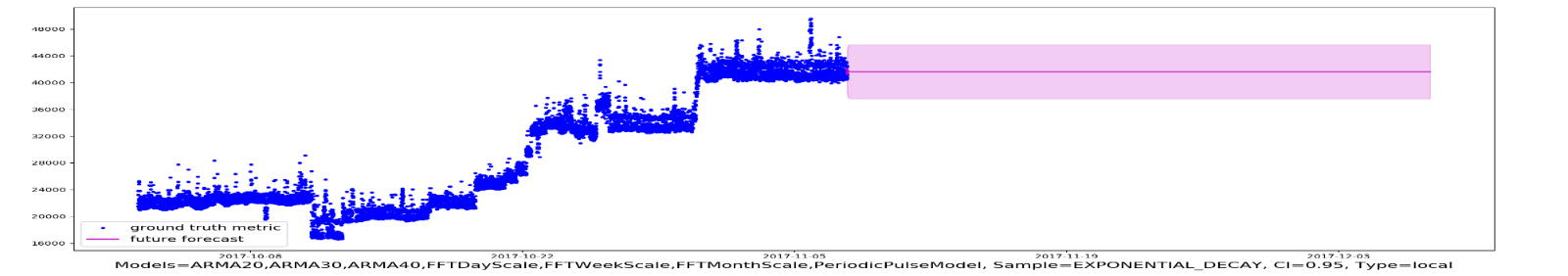
The projection algorithm is based on ARIMA, DFT, Spike and Plateau models. A year's worth daily aggregated (currently average) data is used, with more weight given to more recent data (this feature is called exponential decay). A limitation is it won’t handle workload with annual cycle.

Workaround

If you do not have 3 months and just need an overall sizing, consider using the 97^th percentile value. Why 97^th percentile? It's based on standard deviation principle. Two Standard Deviation away from the midpoint equals to 95%, and 3 Standard Deviation = 99.7%. 97^th percentile hence provides a good balance between 2 SD and 3 SD. By and large, it captures just the right amount of peak and outlier.

Utilization

It reflects the actual, live usage of the resources. If utilization is high, it does not matter if the overcommit ratio is far below your target, the cluster is full.

If utilization is low and won’t go high for foreseeable future, that is not a good thing. Unless it’s a newly provisioned object that is yet to grow to its full usage, or disaster recovery protection, that indicates wastage resources.

How should we fit wastage in the utilization model?

The following is my recommendation. I divide the capacity into 10 equal chunks. That means the usable capacity is green when it’s around 40 – 80% used, with ideal target of 80%

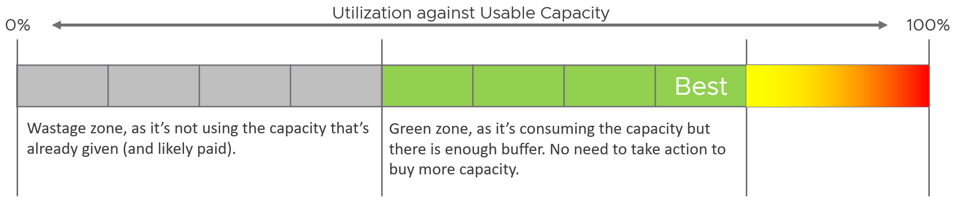
What is the challenge of above implementation?

It’s only applicable for utilization-based capacity. It is not applicable in:

• Reservation. Low reservation does not mean wastage.

• Allocation. It is not something “real”.

• Contention.

This means wastage cannot be used in the Capacity Remaining (%) metric as this generic metric may represent other dimensions.

Reservation

Just because you set a reservation does not mean it’s actually consumed. Reservation that is not yet consumed impacts capacity but not performance. Using a restaurant analogy, if all your tables are reserved but only 20% turns up, you have 0 capacity left but can easily serve all customers as the real demand is only 20%.

From the above you can tell that the demand metrics should not include reservation. On the other hand, you do need to calculate your restaurant capacity. That means you need 3 metrics

• Utilization

• Reservation

• Sum of individual consumer Max (utilization, reservation). This is the metric you should use as the demand.

Let’s take an example of a restaurant with 2 floors.

• The 1^st floor is 100% filled up with diners.

• The 2^nd floor is 100% reserved.

What’s your capacity left?

The answer is 0%. You can’t take any more customers unless they are reservation holders.

Applying the above to vSphere, how do you know who are the reservation holders that are yet to consume what they are entitled to?

For compute, those are VMs already powered on but have not consumed CPU and memory at their reserved threshold. When you get to the actual metric, you will notice there is some complication we need to take care.

VM reservation has a positive impact on the VM performance, but a negative impact on the cluster capacity. It places a constraint on the DRS placement and HA calculation.

Reservation complicates operations because of 3 reasons:

• It has 2 parts: allocated and used.

• Resource Pool and its children VMs can have independent settings.

• Reservation and Utilization need to be accounted together.

For storage, those are thin provisioned VMDK files that are yet to grow to their full size.

Use Cases

When do you use reservation?

I only see 2 use cases. Let me know if you have others:

• To be more conservative with capacity.\

  You want to manage the risk of performance problem from over provisioning. You can’t use the demand counter as the actual demand is not high enough.\

  Total reservation from all running VMs cannot exceed cluster capacity. As a result, this this creates a suboptimal cluster as VMs do not use the entire assigned memory at the same time. The working set is typically much as smaller as the purpose of memory is cache VM Performance

• To give different performance to higher class of service.\

  You’re running mixed class of services in the same environment. To protect the higher-paying consumer, you give them higher reservation. Take note the correlation is not perfect. There is no deterministic correlation between VM reservation and VM performance. A VM CPU Ready does not improve 2x because you increase its CPU reservation by 2x.

Implementation

Now that we’ve covered the theory, where do you set the value? Do you set at VM level or at resource pool level?

Frank Denneman recommends in this blog article that you “create a resource pool and set a reservation at the RP level. If a reservation is set at the VM object-level it has an impact on admission control and HA restart operations (Are there enough unreserved host resources left after one or multiple host failures in the cluster?”

A limitation of the above is the reservation is not tied to the VM. If you operate a multi-cluster load balancing, ensure all member clusters have consistent settings.

Allocation

The total demand could be more than the visible demand, which is the active load that is consuming your capacity. There is demand that is not yet visible, because it has no utilization at present. Use the Allocation Model and buffer settings in VCF Operations to cater for this invisible demand.

The other use case for allocation is showback and reporting. There are typically restrictions such as contractual obligations or SLAs that mandate capacity shall not be overcommitted beyond an agreed upon ratio. Note these restrictions are usually non-technical.

Allocation model is less relevant when utilization or reservation is high enough that you worry about them more than allocation.

Allocation model also has usable capacity concept. Deduct the hypervisor overhead. This means VMkernel, vSAN, NSX, and vSphere Replication must be deducted from total capacity.

Invisible Demand

Rare Demand	This can wreak havoc in a shared environment. A group of highly demanding VMs can collectively impact overall performance of the cluster or datastore. An example of this is annual sales. In this case, the capacity team should set an appropriate overcommit ratio and drive by allocation as the demand is low most of the time. A rare part of sudden demand is disaster, like stock market crash. It can’t be predicted. Whether your CIO wants to pay in advance for such rare thing is a business decision, not within the call of Capacity Planner.
Unexpected Demand	Many critical VMs are protected with Disaster Recovery. During a DR drill or actual disaster, this load will ‘wake up’ and consume. You should consider the Site Recovery Manager Recovery Plans into your capacity. Be careful with the complexity as 1 Recovery Plan can have many Protection Groups, yet 1 Protection Group can be included in many Recovery Plans.
Potential Demand	Many newly provisioned VMs take time to reach their full expected demand. It takes time for the database to reach the full size, the user base to reach the target, and the functionalities to be complete. Newly provisioned VM tends to be idle (which can be months) and may suddenly grow. If you have many of them, plan for their eventual size.
Unmet Demand	There are 2 parts to it: inside the VM and outside the VM. If the VM is undersized, the unmet demand will not be visible to the underlying infrastructure. Unless that is intentional, it is wise to include undersized VM in the cluster capacity monitoring. The visible part of unmet demand becomes part of IaaS KPI and SLA, covered in Performance Management chapter.

Limitation

The allocation model has the following limitations:

VM Size	VM size is not considered in the overcommit ratio. It assumes that scheduling two monster VMs is as easy as scheduling many small VMs. The ESXi scheduler can juggle higher number of small VMs than a few large ones, especially if they peak at different times. Utilization is completely ignored. The consumer part is simply based on the configured amount. In cases where there is additional workload, the allocation model can report lower capacity consumed than actual.
Overhead	Any form of utilization is not considered, including consumption because of virtualization. For example, software-defined storage such as vSAN actually puts the availability protection data in the same datastore with the actual data. So you end up with double the consumption inside the datastore.
IaaS Workload	Agent VM is included as part of demand as it takes the shape of a VM, although it tends to use local datastore.

Overcommit

Overcommit is the main technique to reduce cost of shared infrastructure or shared service. So long the contention (real and risk) is acceptable, it reduces the cost to everyone. In daily life, queueing or waiting for service is common.

As a cloud provider, if you do not overcommit, you may not be able to compete on cost. Public cloud players (e.g. AWS) uses 1:1 overcommit for CPU but they count the thread (not just the core). They do not overcommit memory.

Some customers do procurement planning based on overcommit ratios. A comfortable overcommit ratio is determined, and that’s what is used to project utilization into the future. The overcommit ratio is intended to be a rough estimate of utilization, e.g. 5:1 CPU overcommit ratio means that on average each vCPU should only run 20% utilization else you will have contention.

Consider your SDDC overhead. Your overcommit ratio is smaller if you have kernel modules such as vSAN and NSX. For example, if VMkernel takes up 4 cores and 32 GB of RAM, deduct this from your capacity first, then you do your overcommit maths.

Cluster Capacity Planning

How do we put together the utilization, reservation, allocation and contention into a real-world example? Can this example include 3 class of services (gold, silver, bronze) for a more realistic implementation? Mixed Class is unfortunately common due to budget & environmental constraints.

To start, we need to quantify the relative value of gold vs silver vs bronze. Keep it simple, so it’s easy for tenants to understand the business values of each.

I recommend a 2x gap. It’s easier to explain to senior leadership and application team. Operationally, it’s easier to manage at scale than 1.5x gap or 3x gap.

2x gap means gold class is 2x better than silver class, and silver is 2x better than bronze. To achieve this promise, you put in place techniques such as reservation and allocation. You also guard the performance and keep the headroom accordingly.

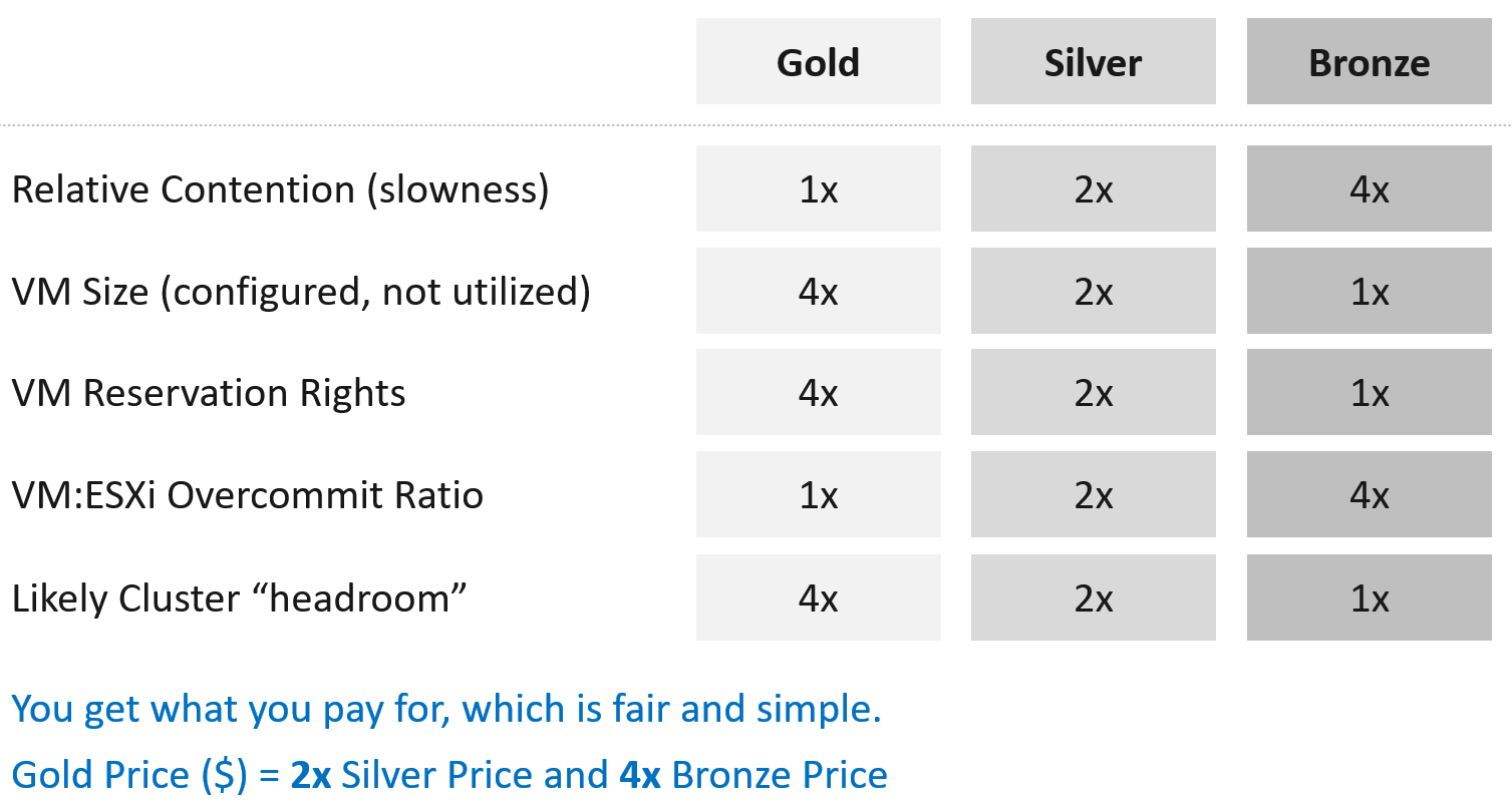
Separate what you promise (or sell) and how you deliver that promise.

• To the tenant, the gold class is 2x better than silver class. The chance of encountering contention is 0.5x silver. This is what you sell.

• You prove to the tenant that you assign 2x reservation, have half the overcommit ratio, and has 2x the headroom. These 3 are the techniques as you can’t directly guarantee contention is half.

How do you implement the above technique?

The following table shows an example of. Notice the consistent 2x gap.

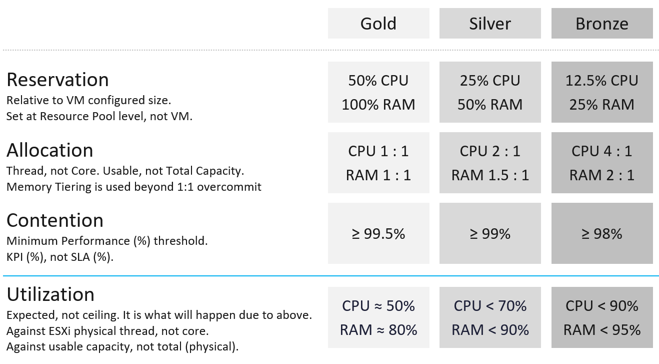
Why is Cluster overall utilization put at the bottom, with a blue line?

Because that is not an input, but an output. It is what likely happens when you set reservation and allocation.

Reservation

This is the only mechanism to protect higher class VM from lower class VM. For example, gold VM is priced 4x than bronze VM because it is entitled to 4x reservation.

Take note reservation is measured in Hertz, not vCPU.

Allocation

Allocation is only counted when the VM is powered on.

It is relative allocation, measured againsts usable capacity.

The CPU is based on thread, not core. So take note the performance degradation.

Take note the number for memory includes memory tiering, a new feature in vSphere 8. The overcommit is based on the physical RAM, meaning it does not count the NVMe device.

Contention

Contention means the cluster KPI, not the cluster SLA. The reason is the context is cluster capacity. You don’t declare the cluster full just because of a one-time performance issue.

Because if the cluster is unable to serve existing workload, capacity becomes 0, regardless of the other 3 numbers. Performance was covered in-depth in the previous chapter.

Why is the performance number lower than the performance SLA?

Because it is not the same number. This number is measured on a daily basis, not monthly basis. This means there is a 30x less margin for error. For example, Silver has a target of at least 99% per day, leaving only 14.4 minutes to fall below expected performance.

Utilization

It is relative utilization, measured againsts usable capacity. However, there is a limitation as the hypervisor overhead cannot be excluded due to dynamic nature.

For Gold, since you do not overcommit, there is a high chance that the utilization is well below 60%.

For Bronze, since you overcommit, the utilization becomes the upper limit. Do not go beyond this threshold as you run a risk of contention.

Stop Provisioning Threshold

As SLA is calculated at the end of the month, it’s a lagging indicator. It’s only useful for business reporting, not proactive operations. To complement it, you need to implement an early warning system that tracks in real time (or maximum every 5 minutes). You need to know when to stop provisioning, as you don’t want to make the matter worse and eventually breach SLA.

In fact, knowing when to stop provisioning is also too disruptive for your operations, if VMs are provisioned via self-service. What do you do for VMs already in the queue of being provisioned?

You need a predictive metric, a leading indicator showing that the risk is getting higher. This enables you to still provision those VMs in the queue, or better still give 1 week worth of heads up.

Class of Service	Stop Provisioning	Early Warning
Gold	When overcommit reaches 1:1	Not applicable, as there is no overcommit. Use the actual allocation to start procuring new capacity.
Silver	When any VM in the cluster experiences VM Contention >1% in any given 5 minute	Cluster Consumed > 95%, or Cluster Balloon > 1%, or Cluster Swap + Compress > 0%
Bronze	As above	Cluster Consumed > 95%, or Cluster Balloon > 2%, or Cluster Swap + Compress > 1%

Template

I’ve created a Microsoft Excel spreadsheet to help you plan capacity based on the above model. Download here.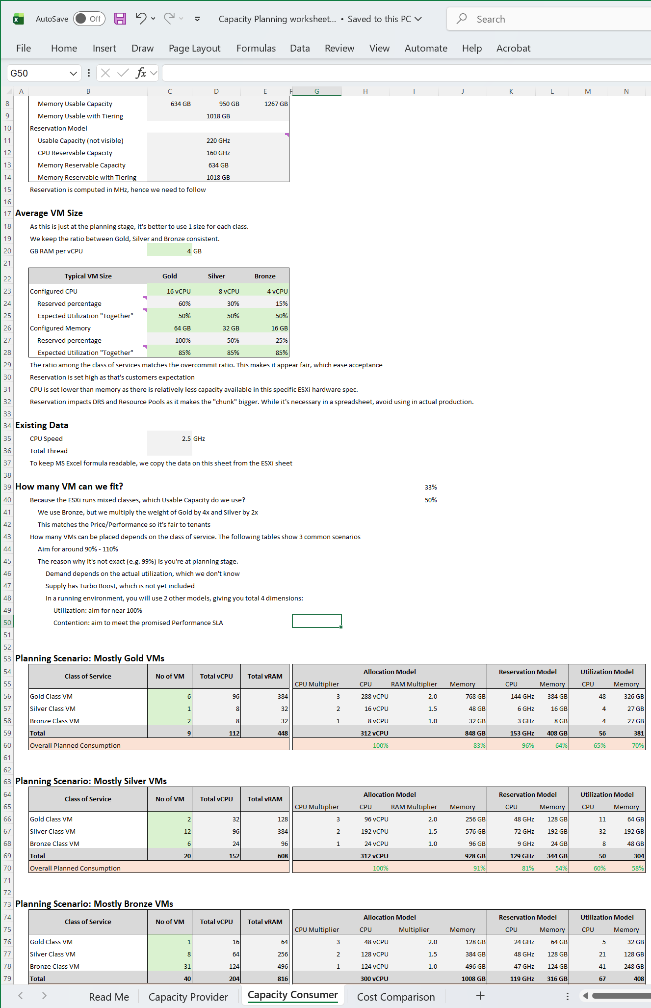

Once you open the spreadsheet, the first thing you need to confirm is the size of your ESXi host.

The spreadsheet comes with default values that I think provides a good balance between cost and size.

Reclamation

It is only applicable when VMs are free. When VM is the main source of budget for IT department, the responsibility to reduce VM cost will naturally shift to the application teams as infrastructure team will not want their budget reduced.

Reclamation delivers many benefits, and some of them are listed below

	Area	Benefit
Unused VM	CPU Memory Storage	This delivers the highest benefit, but it’s also hardest to find as the VMs may not be idle nor undersized. They appear like an active VM. Improve on the underlying IaaS capacity and performance. Savings on storage only happen when you delete the VM.
Oversized VM	Memory Storage	VM Performance. Especially if Guest OS does a lot of CPU context switch and VM size exceeds whole box total core counts. The rest of benefit is the same with Idle VM as the portion you’re reducing is idle.
	CPU	The oversized part is idle. So it only benefits allocation model.
Idle VM	Memory Storage	Cluster Capacity, especially if you use allocation model. Cluster RAM as idle RAM pages tend to occupy ESXi memory. One quick way to free up is to reboot the VM. Negligible savings on CPU demand as idle loop hardly occupies real CPU cycles. Savings on storage only happen when you delete the VM.
	CPU	Idle VM only saves you from allocation model.
Powered off VM	Storage	Datastore Capacity
Orphaned VMDK	Storage	Datastore Capacity. Does not impact cluster capacity
Snapshot	Storage	Datastore Capacity.
Unmapped	Storage	Datastore Capacity

There are 5 areas of reclamation, from the easiest to the hardest. Naturally, the logic differs for each.

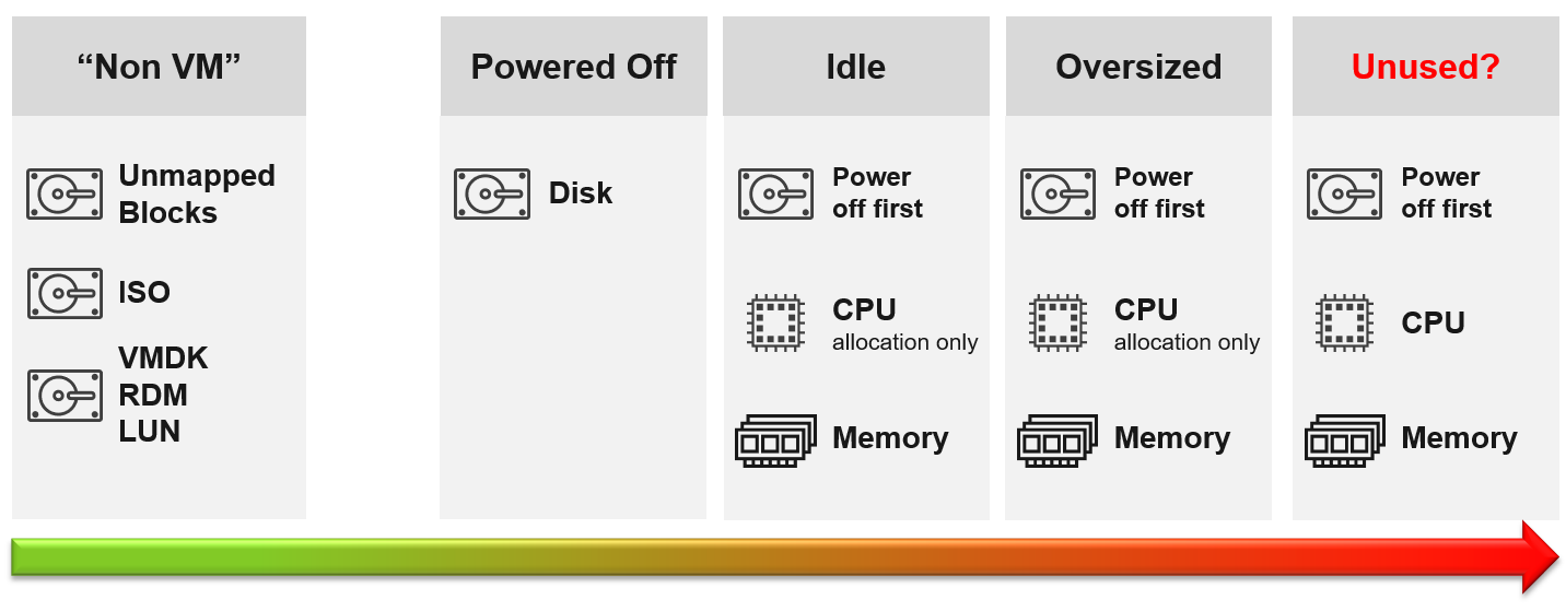
Non VM files are the easiest, because they are not owned by someone else. They are yours! Non VM objects, such as templates and ISOs should be kept in 1 Datastore per physical location. Naturally, you can only reclaim Disk, and not CPU & RAM.

An orphaned file is a file in the datastore that is no longer associated with any VM. Orphaned VMs and orphaned VMDK’s are not even registered in vCenter. If they are, they may appear italicized, indicating something wrong. They may not have owners too.

For orphaned RDM, look from the storage array if there is any ESXi mounting it. You need an adapter for the specific storage you want to monitor.

Snapshots are not backups, and they do cause performance problems to the VM if kept for extended periods of time. Keep them only for the purpose of protection during change. Once the change is validated as successful, keeping the snapshot does a disservice to the VM. A Snapshot is easier to reclaim, hence VCF Operations lists them separately.

Reclamation Approach

Active VM is politically the hardest, as they serve business workload. Focus on large VMs first. Take on CPU and RAM separately as they are easier to tackle when you split them. Divide and conquer. If you reduce both, and application team claim performance impact, you need to restore both. Claiming CPU and RAM from small VMs can be futile, regardless of idleness. An idle VM with one vCPU cannot be further reduced. Focus on the large VMs, for the reason covered here.

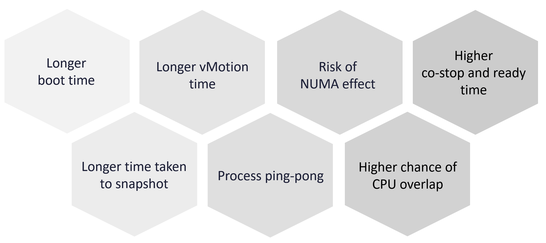
Focus on Monster VMs

When reducing oversized VM or powering off idle VMs, focus on large VMs. Let’s take an example for comparison:

• Reduce 20 large VM. Average reduction is 10 vCPU.

• Reduce 100 small VM. Average reduction is 2 vCPU.

In both scenarios, you reclaim 200 vCPU. But the large VM option delivers more benefits and is easier to realize. Here is why:

• Every downsize is a battle because you are changing paradigm with “Less is More”. Plus, it requires downtime, which requires approval and change request process.

• Downsizing from 4 vCPU to 2 does not buy much nowadays with >20 core Xeon.

• No one likes to give up what they are given, especially if they are given little. By focusing on the large ones, you spend 20% effort to get 80% result.

• Large VMs are also bad for other VMs, not just for themselves. They can impact other VMs, large or small. ESXi VMkernel scheduler has to find available cores for all the vCPUs, even though they are idle. Other VMs may be migrated from core to core, or socket to socket, as a result. There is a counter in esxtop that tracks this migration.

• Large VMs tend to have slower performance. ESXi may not have all the available vCPU for them. Large VMs are slower as all their vCPU have to be scheduled. The counter CPU Co-stop tracks this.

• Large VMs reduce consolidation ratio. You can pack more vCPU with smaller VMs than with big VMs.

Powered Off VM

Compared with orphaned VMDK, Powered Off VMs are harder to remove, as there is now an owner of the VM. You need to deal with the VM Owner before you delete them. This is where tagging them with the owner email or Business unit would have been useful. We discussed proposed tagging in Chapter 1, specifically here.

There are different techniques to define power off:

• Non Stop. In this technique, you want the VM to be continuously powered off. A quick power on to check something in the VM will remove the VM from powered off list.

• Percentile. In this technique, you can turn on the VM for a short period of time.

Each technique has their own pro and cons. VCF Operations use the non-stop as it is safer.

Powered Off as Brake

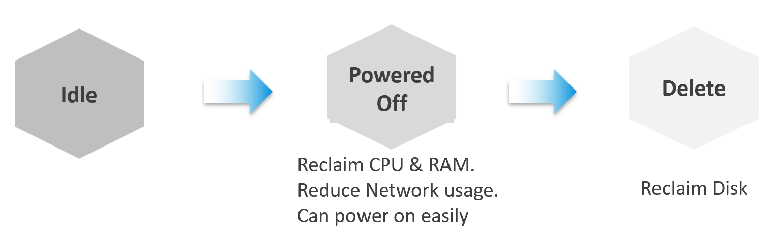
Why do cars have brakes?

So they can go faster!

Take advantage of Powered Off as the brakes for your Idle VMs. If you treat Idle and Powered off as 1 continuum, you can power off the Idle VMs earlier. You get the benefit of CPU and RAM reclamation. It’s a safer procedure too, as you can simply power it back on if you find that the VM is actually being used.

One major caveat if you do this, is the average utilization of the remaining VMs in the cluster becomes higher. As a result, you may not be able to achieve the overcommit ratio needed to break even.

2 Sides of a Running VM

There are two reclamation formula for running VM (idle or not). The formula is complex as it has 2 different stages:

Before	Determine if the VM falls under the category. For example, does the VM qualify as an Idle VM? This should look inside the VM, as that’s where the workload runs. Measuring at the ESXi level could yield incorrect results because: Some metrics include loads not generated by the VM that are charged to the VM, such as vSphere replication and vMotion. Some CPU metrics affected by power management.
After	Determine what can be reclaimed. Since what is being reclaimed is ESXi resources, the usage inside the Guest OS is irrelevant. The queue inside the Guest does not impact the hypervisor, so there is nothing to reclaim at the ESXi layer. All metrics are from ESXi. Guest OS metrics are not applicable as we’re not reclaiming from inside the Guest.

So you need to apply 2 different types of logic.

Idle VM

By definition, idle means it’s not doing useful business workload. A VM that is doing only non-business workload (e.g. AV scan, Windows regular update) should be considered as idle. This non-business workload is hard to detect via unless you have process-specific whitelisting. This is also not fool proof as some non-business software uses Windows or Linux system services as proxy.

Idle VM is a great target, as you can now claim CPU and RAM when you power them off. You cannot claim disk yet as you are not deleting them yet. Take note that you are not reclaiming real CPU cycle as it’s idle to begin with. Idle VM does not actually consume any ESXi CPU cycles. So reclaiming a 10 vCPU VM running only 1 vCPU does not give you 9 vCPU. You are reclaiming blank air. For memory, you will reclaim real ESXi memory as idle VMs tend to have its consumed memory remained on ESXi.

Idle VM has a default threshold of 100 Mhz. This means 5% utilization in a single vCPU VM running on a 2 GHz ESXi. This also means 0.25% on a 20 vCPU on the same ESXi. The reason for static is idle by definition is absolute, not relative to the VM size. Oversized VM is relative.

While a VM uses CPU, RAM, Disk and Network, we only use CPU as a definition for Idle. There is no need to consider all 4, and require all 4 to be idle, because they are inter-related. It takes CPU cycles to process network packets and perform disk activity. Data from the network card and disk must be copied to RAM before processing, and the copying effort requires CPU cycles.

Take note of a corner case limitation of VM with runaway CPU, where CPU is high but no meaningful memory access, network transmission (TX) and disk processing. Idle VM will fail to detect it. It’s a corner case, hence I think it’s not worth the complexity. Also, the CPU runaway typically happens on a process, which likely a single threaded. Use the CPU Usage Disparity (%) metrics to detect that.

Idle has to be defined so it’s measurable and not subjective. Declare it as a formal policy so you don’t end up arguing with your customers.

VM that is rarely used can appear idle, if you measure idleness over a long period of time. For example, if a VM is only productive (from business viewpoint) for 2 hours a week, that means the remaining 166 hours should be classified as idle. That’s 98.8% idle.

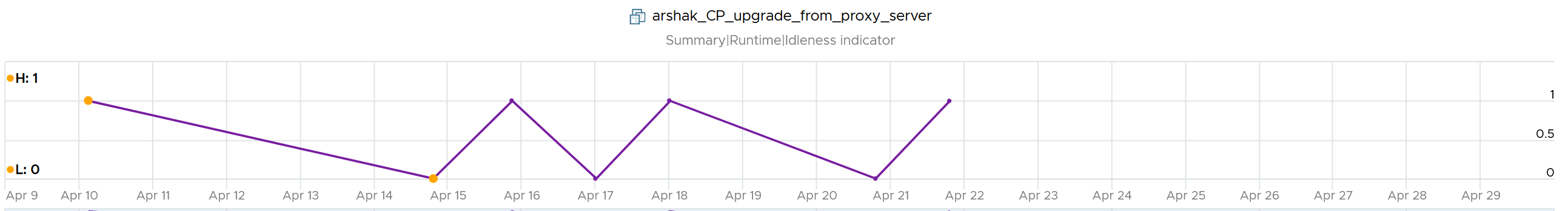
To counter the above, you want to evaluate idleness on a daily basis. A VM has to be idle every single day for ‘N’ number of days. This daily calculation is stored in the counter Idleness Indicator. It is a rolling counter. That means it is calculated every 5 minutes, but each value takes the last 24 hours of data. This is better than calculating only once a day so that VM does not have to wait before it gets declared as idle or not.

As you can see in the following example, its value is only stored if there is a change. This makes it easier to see when and if it changes.

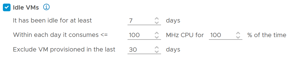
Now that you have it daily, it’s a matter of rolling up to the whole period (default value is 7 days). We set the value to just 7 days so you can see the calculation result within a week. Note that we set to 100% and we ignore newly provisioned VM.

Think of the various situation before extending from 1 week. For example, a VM has been in production for a few years. A new version of the application has been developed, and this VM is being decommissioned. The VM goes idle. As the application team does not inform infrastructure team, the VM will take at least 7 days before it’s marked as idle. If you change that to 1 month, it will take longer.

On the other hand, a month-end VM that processes payroll can be idle for 29 days.

The counter that covers the whole period is called Reclaimable Idle.

It is a daily counter, that’s set to 1 (true) if the VM meet the idle criteria.

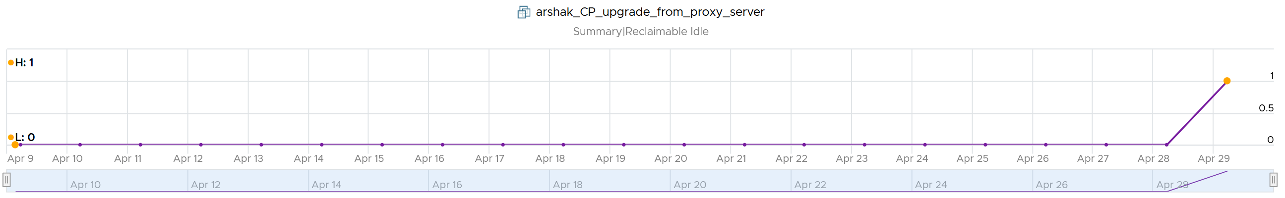
To list the idle VM, you need both metrics to be true.

Why can’t you just use Reclaimable Idle?

Because it’s a daily counter. You can mistakenly assume a VM is idle even though it’s recent activity shows it’s not idle anymore.

In some environment, it can take time before a newly provisioned VM is used. Check the creation date of the VM before powering it off.

Have we got all cases covered?

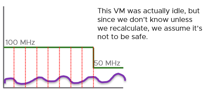
Nope. There is a corner case, where you tighten the definition (say from 100 MHz to 50 MHz). What was Idle may no longer qualified for idle. We can recalculate the daily metric, but this consumes performance. So to be safe, we will restart again from Day 1. So if the Idle Window is 2 weeks, customers have to wait 2 weeks.

Oversized VM

Oversized VM has a different logic than idle VM since the Idle VM definition does not depend on the size of the VM. The Idle VM definition simply measures if the VM is generating enough workload or not. Idle is about GHz, while Oversized is about %.

Oversized VM depends on the size of the VM. A 64 vCPU VM running 7 vCPU is oversized, while an 8 vCPU running 7 vCPU is not.

VM Is undersized	Calculated based on CPU & RAM total capacity and recommended size values. If for at least one of the containers (CPU or RAM) the recommended size > total The lowest value for increasing the CPU is 1 vCPU and for memory is 1 GB
VM is oversized	The VM is oversized if it is possible to reclaim a CPU or Memory. Calculated based on CPU & RAM total capacity and recommended size values.
VM Reclaimable CPU	Calculated based on socket counts and core counts of VM = Minimum (( reclaimable Sockets * cores Per Socket + reclaimable Cores In Remaining Sockets), CPU Core Count - 2) Will not suggest the reclamation if the CPU Reclaimable value < MHz Per Core value
VM Reclaimable Memory	= total Capacity – recommended Size Must be ≥ 1 GB and the remaining capacity after reclamation should be ≥ 2 GB

Limitation: the implementation in VCF Operations is based on projection, not a mere 5-minute or 1 day data. So if you power off an oversized VM, it remains considered as oversized until it passed the definition.

Cost of Oversized

More CPU, memory and disk do not translate into faster performance. In fact, it carries additional overhead.

TRIM and Unmap

When Guest OS delete files or parts of it, it does not replace the value with 0 and just leave the block. This is more efficient and also enable recovery. But this cause the underlying VMDK to grow. The same thing happens at the array level. This is where Trim and Unmap come in.

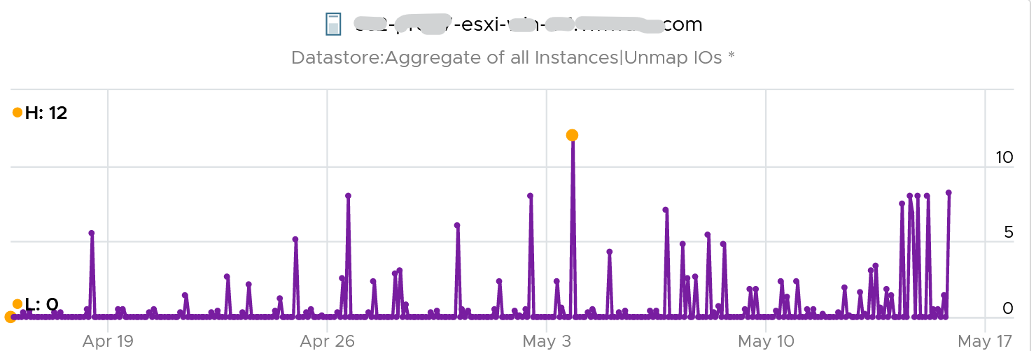
VCF Operations tracks the unmap operations via 2 metrics at ESXi Host. The first one is Unmap IO, which tracks the number of unmap SCSI instructions. For example, if the value is 100, that means ESXi has sent 100 requests of unmap to its datastore. So think of it like IOPS, except the IO is not writing/reading actual block, but more of a request to delete (unmap) the block in the back end array. The value is the sum of 20 seconds since vSphere reports per 20 seconds, then averaged over 5 minutes. In the example below, you can see the host sends unmap commands frequently in the last 30 days.

The second metric is Unmap Size, which tracks the total unmapped space from the operations above. The value is shown in MB.

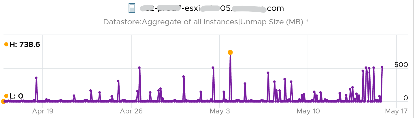
You can track both operations on each datastore, but you can’t aggregate them per datastore.

For further reading on TRIM and Unmap in vSAN, read this detail article by Patrick Kremer.

The problem only happens on thin provisioned disk. So if you want to check how much space you can reclaim, create a view that compare the value inside the Guest vs the value shown at VMDK level.

Unused VM

Unused VM is not idle, but they do not provide business value anymore. The application team may have stopped using it, but left the application running just in case they need in the future. The VM is not idle as it still generates CPU activity. The activity can be business workload, IT workload, or both.

This makes unused VM much harder to find, as what works for VM 00001 may not apply to VM 10000.

The IT workloads take many forms. Guest OS upgrade, Guest OS patches, and application patches can be 3 different workloads with different patterns. VMware Tools patches, anti-virus scan, intrusion detection scan and agent based back up are other common examples. In an environment with high security, there can be many security related agents running. Or worse, they can be agentless, executed via network.

Business workloads can be batch jobs, reports or monitoring. No one is using the application anymore, but the application continues running. It could be generating report and send email to someone who just ignore that emails. This is harder to identify than the one running pure IT workload as it’s more unique.

Unused VM is hard to detect as the infrastructure team lack the business context, and the patterns vary widely. The owner verification is required before you power off the VM. This is why it’s important to have ability to relate a VM to a department or owner. We discussed the necessity of business-centric infrastructure in Part 1 Chapter 1.

There are some checks you can do to find the unused VMs when their CPU usage is not low. Find VMs that exhibit multiple of these behaviours. Take note that each of these can be false positive, so you need multiple of them for more accurate conclusion.

Configuration

Configuration is easier to interpret than utilization, as they tend to have clear cut rules. The following list some configuration items you can consider.

Isolated	It’s no longer connected to a virtual NIC, so it’s not communicating with other machines.
Guest OS	It’s running older version, especially those nearing End of Life. It indicates the application team may have written a replacement applications running somewhere else. Running old version of Windows, Linux and/or Kubernetes. Expired license. Temporary license.
Application	It’s running older version, especially those nearing End of Life. It’s running application that you no longer license. In this case, there is urgency to power it off. It’s running without license, or with evaluation license, or expired license. It has no business application installed. Just base OS + IT security applications.
Owner	It belongs to a folder in vCenter that is no longer owned. Unable to figure out the tagging for the VM. Request to contact the owner has gone unanswered. Owner has changed organization.
Report	The application is no longer listed in any of the reports to the department owning it. This could be performance report, capacity report, compliance report, chargeback report, etc.
Location	It runs on a cluster that is due for decommission. It is stored in a datastore, that sits on an array that is due for decommission. Its folder has names like “old”, “decommissioned”, and “archived”.
Relationship	The VM is talking to other VMs. You can check which services is talking at which port. Check what services it’s using over the network. This is useful for VMs in the cloud, which uses cloud services from AWS, Azure, etc. As these neighbors could also be unused, using this alone is not reliable.
Alert	Alerts associated with VM have disabled.

Utilization

CPU	While usage is not idle, or even high, it’s the same CPU. There is very little context switch, indicating the same processes are running. If the CPU Usage Disparity (%) metric is stable, that indicates constant run.
Memory	While the In Use metric is high, it’s passive. There is lack of paging, both in and out.
Disk	While IOPS and throughput are not low, its filesystem is stable, rarely changing in both size and activities. The IOPS and throughput also eventually form a pattern over the long run.
Network	The network it belongs to is no longer reachable, or has been isolated. That means access to it is non-existent or highly restricted. The VM sends very little packets out, indicating it is not talking much on the network. At the same time, it’s only talking to a fixed and small group of other servers. Take note that secure applications that store data typically are restricted.
	It belongs to a VLAN that is due for decommissioning.
Log	The amount of logs or Windows Event is much lower relative to its peers. The pattern is also predictable over time.

Other Signs

No login	No one has ever logged into the Guest OS, be it from UI or the console (e.g. SSH into Linux) for a long time. If user log in, it’s for a very brief period of time.
Process	It’s the same set of processes that are running. The number of processes also remains steady and predictable. The process that takes up the most CPU is not business software. It’s system process or IT application.
Availability	It never gets rebooted, or it gets rebooted often. Essentially, it seems like no one cares about its state. Reboot happened during business hours and no one complained.
Performance	Severe performance issue and you don’t get a complaint. If someone owns it, you will get a formal ticket if the performance is terrible for a long time during business hours. At night, a VM can experience slowness for 1 hour and no one may notice.

Bottom line, what can you do if you are unsure?

You’ve announced to everyone that the VM would be deleted if no one claims it repeatedly, yet no one replied. Anything safer you can do than powering off the VM, as powering off disrupts the running process and close opened files? Powering off does not guarantee that it can be brought online successfully.

You have 2 choices:

• Disconnect it from the network. This makes the VM isolated, without shutting down the application. If it’s used, the VM Owner will know it.

• Apply CPU limit to it. This slows down the VM. The VM Owner will feel the impact and complain it’s slow.

When you do that, ensure you tag the VM or move them into a “Unused VM” folder. If these unused VMs spans multiple vCenter servers, use VCF Operations custom property. If there are many of them, create a dedicated dashboard so you can see them at a glance.

Annual Stocktake

Unused VM is hard to detect. If you don’t have the VM owner, perform a stocktake on those unidentified VMs.

Stocktake is applicable if your IT business is not profit oriented. This means it applies to internal IT department even though you have chargeback as you aim to be a good corporate citizen.

The stocktake actually starts from Day 0, where VM is being requested. Make expiry date mandatory, to catch those temporary VMs. For permanent VM, set it to 1 year. If you set beyond 1 year, you increase the risk of change of owners and you lose the contacts. Reorganisation can result in the department or team owning the VM no longer exist. What was meant to be permanent VM suddenly becomes unused VM.

You need to have a process to keep unused VM in check. Have a simple process so that you can get an agreement from all your customers. As business owners may not know the VM name, include the following information

• Hostname. Take the one from inside the Guest OS, not from vCenter.

• Application name

• IP Address. They may login with IP address and it rings a bell to them.

• Guest OS name and version.

• vCenter Folder name. This should be the business unit it belongs to. See Part 1 Chapter 1.

• 95^th percentile utilization in the last 3 months.

• Any other information and context you think will help them remember it’s their VM.

Rightsizing

What do you rightsize? Not all objects are relevant for rightsizing. Take for example, an ESXi host. Once you buy it, you rarely change the size over the lifetime of the server. Same with datastore and vSAN.

Typically, what you rightsize is VM and Kubernetes.

Let’s dive into VM. Why so many oversized VMs?

Over Provisioning is a common malpractice in real life SDDC for these reasons:

Legacy	Physical machine was P2V, bringing its configuration as it is.
Cost	The price is low for the business paying for the VM. The private cloud is either free or much cheaper than public cloud.
	No progressive pricing. An 10 vCPU VM costs exactly 10x of 1 vCPU VM
Education	The mindset that bigger capacity means better performance is hard to change.
Vendor	Some sizing is dictated by the vendor owning the commercial software. They will not support if you deviate from it.

Challenges

Taking away resources from VM owner is notoriously difficult. The political science part is harder than the rocket science part.

Fear	Will it be slow after the VM downsized?
	You need to prove, using metrics, that there is no performance degradation. What if the slowness is caused by other factors? It is possible that other factors other than CPU or memory were the actual culprit. How do you prove it?
	Solution: Establish a formal and transparent process where VM owners can see their VM performance and usage pattern before and after. The comparison should span 1 month just in case there is month end peak.
Paid For	If the VM was already paid for, how do you position it, so the original size did not look like a mistake by other people in their planning? You don’t want to come across correcting other departments.
	Solution: Project them as the real hero that saves the company, and the infrastructure team as just the facilitator.
Micro Burst	This is the hard part. Some applications have sharp but short CPU bursts. They only last a few seconds, so a 20 second averaging fails to show them.
	Highly volatile burst typically does not apply to memory.
	Solution: Collaborate with VM owners since they have business transaction level monitoring. Use the 2 second metric in VCF 9.1.

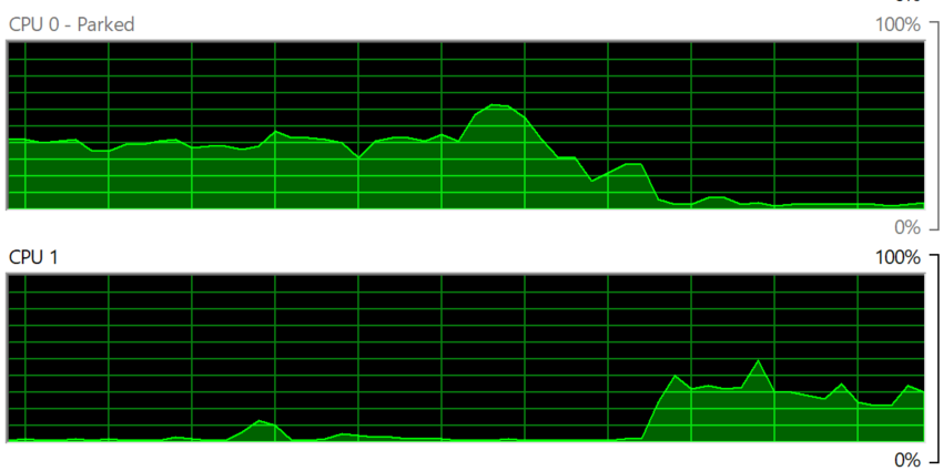
Micro Burst

In the following screenshot of Windows Performance Manager, the 2 CPU shot up to >80% for just 1 – 3 seconds.

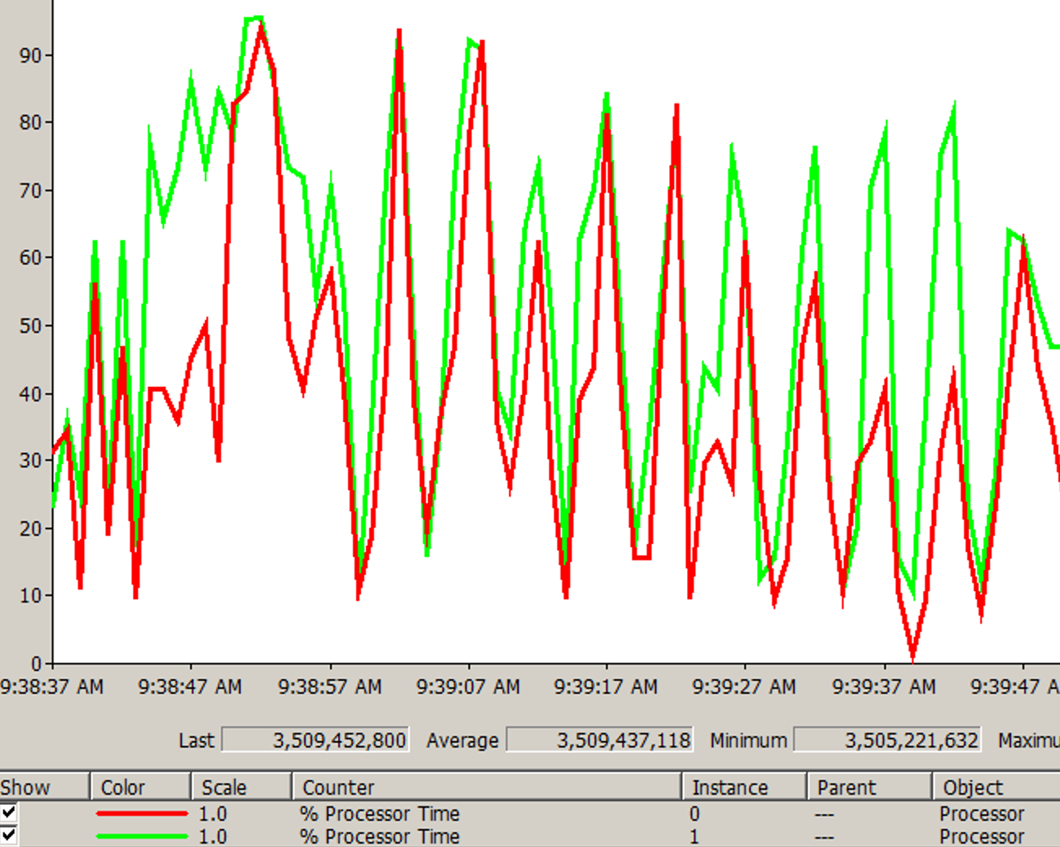
The data point above is per second. If you average the number over 20 seconds, it will show 50%. If you downsize to 75%, you will likely have higher CPU run queue.

There are 2 main approaches to identify the applications:

• By default “No”.\

  The onus is on the application team to inform the infrastructure team that their application has short and sharp CPU burst.

• By default “Yes”.\

  The infrastructure team conducts a company wide scan. Since agent cannot be used, your choice is esxtop, VCF Operations 9.1, or build your own adapter. Since 2 seconds results in high amount of data generated, limit the number to 1000 data points to avoid impacting the system being monitored.

Best Practices

Hardware	Map to the underlying hardware (CPU, RAM) architecture. AMD EPYC and Intel Xeon use an 8-core block.
Performance	Rightsizing is not about capacity. The capacity is there to ensure performance, especially during peak times.
	Solution: Include contention metrics in the formula. For time-sensitive business transactions, measure at this level and Guest OS level. Track contention before and after downsize change to prove that there is no impact. Have a dashboard that any application owner can use.
Collaborative	Agree upfront on the metrics and methods to quantify performance. Ideally do this before relationship turns defensive.
	Agree on the date of the change. Make it a joint execution.
	Solution: Make a dashboard where everyone can see Before vs After for each VM that was rightsized.
Show big picture	While a few VMs may not attract the attention of the C-level leaders, the total may be financially significant.
	Solution: Show a company wide number showing the excess. Report regularly and send it to all stakeholders.
Encourage small	Small VMs are immediately provisioned, available via self service. Larger VMs require more justification and management approval. They are also subjected to regular review of their consumption.
	Solution: Progressive pricing. Discount for small VMs is subsidized by premium pricing of large VMs.
Application-aware	Certain applications such as Java VM and databases manage their own memory.
	Kubernetes Node does not run applications directly. They run containers, which in turn run the processes and threads.
	Solution: Exclude them from the standard formula. Work with the DBA or K8 SRE.

The Big Picture

If you have thousands of large VMs, how do you communicate easily to your senior management that many of the large VMs do not use the CPU given to them in the last few months?

You need to present a convincing chart, that shows the utilization of hundreds of large VMs (which you defined as having > 16 vCPU) every 5 minutes, so a short peak is not excluded in your presentation.

The first thing you need is to create a dynamic group that captures all the large VMs. Create 1 group for CPU, and one for RAM. You then plot their utilization, every 5 minutes, in the last 3 months.

In a perfect world, if all the large VMs are right sized, which scenario will you see: scenario 1 or 2?

Both scenarios show the average CPU utilization of the large VMs.

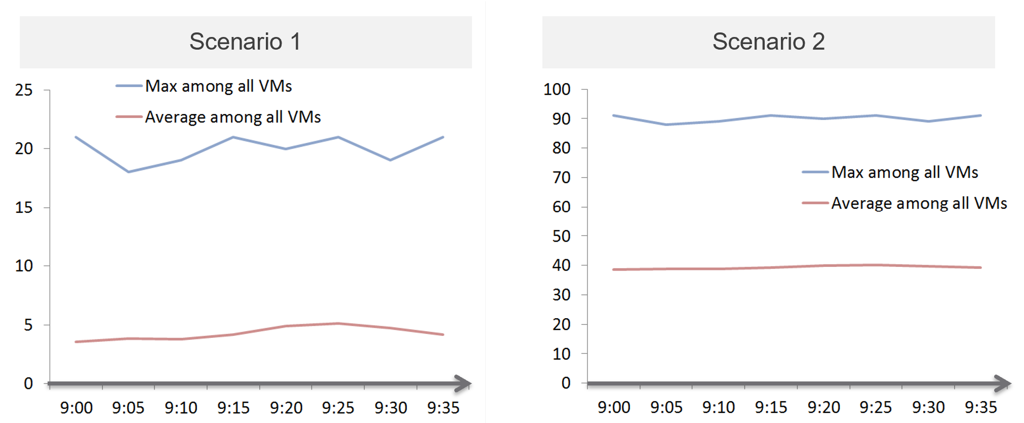
That’s right. Scenario 2.

Because the group has hundreds of members, there is a good chance that one of the large VMs is using the CPU given to it. On average, they should be hovering around 40 – 50%, as at any given 5-minute interval, some may be idle while others may be busy.

The technique we use for both CPU and RAM are the same. I’d use CPU as an example.

Once you create a group, the next step is to create two supermetrics:

Maximum()	Maximum CPU Workload among these large VMs. You expect this number to be hovering around 80%, as it only takes 1 VM among all the large VMs for the line chart to spike. If you have many large VMs, one of them tends to have high utilization at any given time.
	If your Maximum line is constantly ~100% flat, you may have a runaway process. To find out which VM, list the VMs and set the 95th percentile of the time period you’re interested. The runaway VM will be at the top showing 100%.
	If this number is low, that means a severe wastage.
Average()	Average CPU Workload among these large VMs. You expect this number to hover around 40%, indicating sizing was done correctly.
	If this chart is below <20% all the time for the entire month, then all the large VMs are oversized.

Why is it not needed to create the Minimum?

There is bound to be a VM who is idle at any given time.

The 2 line charts show us the degree of over provisioning. Can you tell a limitation?

It lies in the counter itself.

We cannot distinguish if the CPU usage is due to real demand or not. Real demand comes from the application. Non-real demands come from the infrastructure, such as:

• Guest OS reboot.

• AV full scan.

• Process runaway. This can potentially result in 100% CPU Demand if the application is multi-threaded. How to distinguish a runaway process from legitimate high workload is the challenge.

Progressive Pricing

How do you prevent oversized VM to begin with?

Hint: why doesn’t cloud providers like AWS have oversized VM issue?

They have no issue as it’s good for their business. In fact, their profit margin is higher on oversized VM.

One effective solution is progressive pricing. We cover this in Part 1 Chapter 5 Cost & Price Management.

If you do not charge for VM, then you’re left with official approval and corporate policy. For example, the bigger the VM, the higher the approval chain. You can also make the form more complex, needing more justification for monster VM.

Regardless of the pricing, make sure each VM has life span. While they can live forever, they are subjected to annual confirmation that they are still required by the business.

Start Small?

Considering the above problem, how do you prevent the problem to begin with?

One idea is to give every VM a minimal size regardless of their requirements. As this standard is small, majority of VMs will end up needing an upsize over time. So you need to be prepared for CPU Hot Add and memory Hot Add.

There are a few things to consider before taking this approach:

• It goes against the service provider business model. This is classic System Builder, where IT acts as the infrastructure architect, getting involved on VM sizing discussion. Ideally, you use price as your primary lever for sizing, as you may not be familiar with the load of their applications.

• Upsizing logic is more complex than downsizing. You need to consider NUMA impact on performance. The maximum size also depends on the ESXi hosting the VM.

• It can be abused. A synthethic load can be added in the code. Counter this by having a continuous and long-term monitoring.

• Upsizing needs to be more responsive. While application team can tolerate weeks before you downsize their VMs, they probably want their VM to be upsized within the same day. And if performance is affected, they may even ask for it to be done within an hour or so.

Before vs After

Since you’re reducing CPU and/or memory, it’s essential to show the key statistics before and after the changes.

CPU

The overall utilization should remain the same. If the CPU cycles drop (in GHz), increase the share instead of adding back the vCPU.

If the usage was spread across all CPU, the remaining CPU will likely show higher utilization.

If the usage was uneven, the remaining CPU will show similar utilization. In the following Windows machine, the CPU basically took turn to run.

The CPU run queue should not go up. It should remain the same. If it does, check the thread states metric.

The CPU context switch should go up, if the application runs many threads. Ensure the increase is negligible.

Memory

When memory is reduced, you will likely see less free memory, and more active swapping.

If the VM is large and suffers from NUMA, the Local NUMA metric should go up. This should improve performance, especially on memory intensive applications.

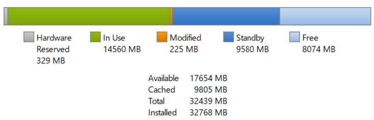
Using Microsoft Windows as an example, you will likely the Available (MB) metric drops. This is fine as the memory is not used. It is not deleted as deleting it serves no purpose as there is no demand.

Other Changes

Changes in CPU and memory utilization can be caused by disk and network demand. Ensure you’re comparing apple to apple by plotting disk IOPS, disk throughput, network throughput and network packets/second.

Logic

Rule	Description
It’s not just utilization	It needs to consider unmet demand. CPU wants to run, but it cannot. Memory has lots of page faults in Guest OS memory.
It’s not just demand	Size base on what the Guest OS needs to perform well, not just base on what it demands at present. Applicable for RAM, where Guest OS can’t operate optimally without buffer. In capacity, we size not just for demand, but also for performance. While we can satisfy the demand for memory with just the In Use, it might come at the expense of performance. The only thing faster than memory is CPU. So make sure CPU is not waiting for data. This is done by caching as much as possible, as it's hard to predict what pieces of data is required by the program.
Includes peak	Consider the busy or peak period, because that’s when the VM needs to work the most.
Consider big picture	A single 5-minute burst is too short a timeframe to determine the entire next 3 months. Consider long term pattern. This alone makes sizing an art, as you need to know the nature of the workload.
Excludes IT load	Exclude the time when the Guest OS is not doing business workload. There are a few IT workloads that cause high utilization. Common ones are Guest OS reboot, Guest OS updates, anti-virus full scanning, agent-based full back up. So long as these tasks don’t prevent the Guest OS from doing useful work, you can exclude them. The exception is when your VM needs to run at these non-business hours too. So it depends on the VM. This is the hard part, as it requires awareness of the footprint (read: process name)

Sizing upwards and downwards should have identical consideration.

• The only difference is they have different boundaries. The lower boundary applies to downsizing, and the upper boundary applies to upsizing.

• For downsizing, Guest OS needs a minimum amount of RAM to operate.

• For upsizing, consider the NUMA boundary. Also, a VM should not be larger than the total number of logical processors on the ESXi Host, else it won’t even boot. In fact, it should be smaller as you want to account for the VMkernel overhead.

As you can see from above, sizing is complicated. And the above is just Guest OS. We have not considered other things that need sizing such as Containers and Business Applications.

The art of sizing has 2 parts: time and metric.

• First, we calculate the value for a given point in time. The correctness of the input value matters, else you have GIGO effect.

• Second, we plot thousands of these values over time, and project it over time. The projection has to consider the peak cycle, meaning it has to be geared towards conservative sizing. It also has to consider the business cycle. If you have annual sales, then consider annual data.

Migration

The arrival of the cloud makes migration more common than before. While the destination differs, the sizing methodology does not. There are many examples of migration. Popular ones are:

• From old DC to new DC.

• From on-premises to cloud. This is typically VMware-based cloud as you can simply move without changing VM. Examples are Amazon VMC and Microsoft AVS

• From Cloud to on-premises. This is typically due to high cost. It’s hard to beat owning with renting if you apply a 5-year TCO. Cloud used to give newer hardware, which is no longer the case.

In the above, you typically change all infrastructure. New server, new network, new storage, new SDDC. You may virtualize network & security by adding NSX. You may also virtualize storage by going vSAN.

Migration ranges from a simple 1:1 to complex M:N migration. It also ranges from a single cut over done over the weekend to multiple migrations lasting years. Destination can be on-prem (e.g. cluster upgrade) or cloud. I’ve seen both directions.

Challenges

Regardless of the migration type and scope, there are some common changes and basic requirements. These could create challenge in the migration project.

Faster Destination

You are using faster & bigger hardware. You have higher CPU speed, more CPU cores, faster RAM, faster storage, bigger network, less network hops, etc. It’s faster by at least 4x compared to the ageing environment it replaces.

And that’s exactly where the problem might start.

A VM that takes 8 hours to complete its batch job may now take 2 hours, all else being equal. So it completes the same amount of work, doing as many disk, network, CPU, memory operations in 4x shorter duration.

So what happens to the VM IOPS? Yes, it went up by 400%, all else being equal.

What happens to VM CPU Usage? It also went up by 400%, as it has to complete the same amount of logic. Suddenly, a VM that runs relatively idle at 20% becomes highly utilized 80%. What was an oversized VM has become an undersized VM.

I call the above as Performance Multiplier. Unfortunately, it’s hard to guess the impact. This is why you are better off testing with a few well known VM first, such as infrastructure VMs or applications that are owned by IT. Examples are email servers, file servers and your Active Directory services.

Because of the above, my recommendation is to keep the VM size. Do not rightsize and migrate at the same time. If you change the size, you will be in the defensive position if there is performance issue.

Different Architecture

The destination could be using software-defined storage and network. Both vSAN & NSX consume ESXi CPU and memory, not to mention storage and network. You must also be aware that certain vSphere disk space counters got affected by vSAN FTT policy.

If you’re migrating to the cloud, take note that the management load and SDDC load, such as vCenter and NSX Edge appliances are also residing on the same cluster. The unique nature of VMware-based cloud migration creates situations that you need to address. For example, you need to watch Elastic DRS if you do not want it to get triggered.

Cost Pressure

How do you typically justify the budget for the new infrastructure, since it’s both faster and bigger?

Yes, you promise higher consolidation. You have more CPU cores, more RAM, so logically you use higher over-commit ratio. As Mark Achtemichuk said in this article, use it carefully.

Since you have to increase overcommit ratio, how do you then prove that performance will not be affected as you drive utilization higher? That calls for a Before vs After performance comparison.

Enterprise IT (read: Infrastructure Team) is also using the opportunity to right-size VM, but VM Owners are against downsizing. How to down-size VM without impacting performance?

Long Migration Project

The problem with project that lasts months is things change. The application may change due to business or technology requirements. The people (application team, infrastructure team, management team) may change and politically this can complicate matter. In large scale project, the inter-DC pipe can be a choked point if large number of VMs on both sides are communicating at the same time. For example, if you only have 10 Gb/s bandwidth for inter-DC, it may not be enough when you have 500 VM on Site A + 500 VM on Site B using the pipe. You essentially only have 10 Megabit/sec per VM. You can try to group the applications, but you can’t control if they change.

This is why I’d rather choose intensity over time. Migration is not one of those projects that are best done slowly.

The following shows an example where the migration takes 6 months.

I drew 1 source cluster and 1 destination cluster. In reality, there can be many to many relationships.

The source cluster has both less capacity (hence smaller area) and slower performance (hence darker color). This is a typically scenario as the new hardware typically delivers faster speed and more space for the same cost.

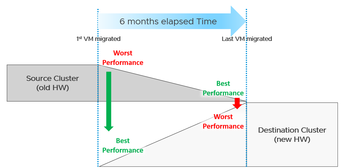
What potential problem did you spot?

This long migration period created an undesirable situation where the first few VMs enjoyed the whole cluster. They could run with 0 contention as there was enough resource for everyone.

Application team felt the responsiveness. Everyone was happy. They might start new features or load the systems even more. Overall utilization went up. So far so good as there was enough capacity.

As more and more VMs get added, the new infrastructure hit the point of overcommit. At this point, the VMs would begin experience contention.

On the other hand, the remaining VMs in the old clusters began to experience less contention. So their performance actually improved. The application team felt good, and started taking advantage of the newly found performance. They begin changing the application or increasing the data size. The users’ expectation also went up as they can do more work. Everyone is feeling more productive.

The last VM to be migrated might get a shock. The performance might actually drop from the end user’s viewpoint.

The above could result in mismatch expectation. This is why SLA matters. You also need to have the SLA agreed prior to the migration. Do not rely on users’ complaint or user-level metrics as that’s beyond your control.

Best Practices

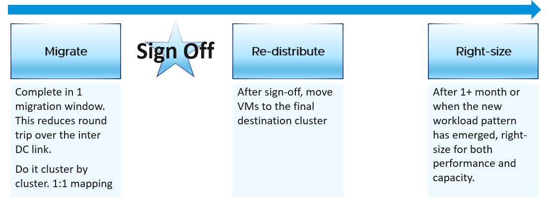
Migration is best done as soon as possible, ideally in one migration window. This minimize inter-DC traffic. For example, if VM 1 talks to VM 2 and VM 2 talks to VM 3, if you somehow forgot to migrate VM 2, you have a ping pong traffic. The latency and bandwidth could cause application performance. So pick the longest window you can get, such as major public holiday or company shutdown.

Migrate 1:1. This means 1 source cluster and 1 destination cluster. Obviously, you exclude the powered off VMs 😊 This makes migration management, and VM troubleshooting easier.

Within a week, get a sign off. Before sign-off, do not allow changes as that can make comparison invalid. Changes include application, business functions and infrastructure.

Do not right-size using the utilization data of the old Data Center. Wait until the new pattern establish itself. I recommend resetting the capacity engine starting date.

Infrastructure Sizing

You are planning a tech refresh for Cluster X. It has 24 ESXi and 1000 VM. You are hoping to reduce infrastructure to 12 ESXi, hence you buy newer CPU, increase the clock speed and add cores per socket. With such major changes, do you consider individual VM one by one, or you do see how they behave as a group?

The answer is the latter, as 1000 VM will not peak at the same time.

Do you consider what happens inside Windows or Linux, or do you see their footprint on your ESXi? The correct answer is the latter, as what happens inside is irrelevant.

Simple Migration

Aim to do a 1:1 migration. 1 cluster to 1 cluster. After you migrate successful and got the sign off, you then move the VMs into their final destination cluster.

If you do this 1:1, your sizing becomes much simpler. You simply add headroom for the next 3 years or so at the cluster level. If your new cluster sports vSAN and NSX, you need to consider their overhead. Speaking of overhead, you also need the VMkernel overhead, which varies.

The issue of you have with the single VM gets amplified here. Instead of dealing with just 1 faster VM, you now deal with many. Even if the workload is identical, since they complete the job in much less time, your workload pattern turns to spiky. What took 1 minute now take 20 seconds. If your monitoring is 5 minutes, your observability is 300 second average. You can have microbursts that you cannot see. This is why using the 20-second peak metrics is necessary.

Be aware of heavy hitters VM. Consider 2 VMs. Both have 16 vCPU. Both are running hot, but one of them is heavy on IO. It sends a lot of network packets and doing lots of disk IOPS. This 2^nd VM has a different footprint on the ESXi. It’s much more demanding. All those IO processing need to be processed by other physical cores. That’s why your sizing should include disk IOPS, disk throughput and network throughput.

Generic Formula

New Sizing = (Sum of VMs Usage x Future Growth x Performance Multiplier) + Overhead

Where:

Sum of VM Usage	It is the chosen number to represent all the data in the assessment period. Ideally, you capture 1+ year so you do not miss annual data. Now that’s ~105K datapoints as there are that many 5-minutes in a year. So what numbers do you pick? If the chart is trending, especially upwards, you need to account that the workload is increasing. So I’d use a projection, instead of simply take say the 95th percentile. The percentile also treats recent data as more relevant. For such large data sets, there can be outlier. Both projection and percentile handle this.
Future Growth	The headroom you need before you top up hardware. So if you buy every year, then you need at least 1 year of buffer
Performance Multiplier	An additional buffer you put to account that faster performance.
Overhead	Virtualization layer, which is vSAN + NSX + VMkernel load. This is the reason why you can’t take your existing cluster load. Your new cluster overhead is different. It’s likely higher as your hardware is bigger, and you may have vSAN and NSX.

Notice something missing?

Yes, it’s reservation. I exclude it as you need to avoid using it. If you want to use it, take the maximum of Usage or Reservation.

Specific Formula

The generic formula we have needs to be applied to each of the 4 elements of infrastructure. CPU, memory, disk and network need to be treated differently.

We also need to apply to specific object. Let’s start with vSphere Cluster as that’s the most common.

CPU	Your main number is in GHz. You support that with another number, in vCPU. For vCPU, the performance multiplier does not apply as you maintain constant. Usage is based on allocation. Overhead is expressed in physical core, so you apply it on the Usable Capacity instead. Allocation Sizing = (Sum of VMs vCPU configured x Future Growth) Make sure this number is within your comfort level.
Memory	You only have 1 number. It’s in GB. Performance Multiplier does not apply to memory as it’s just a storage space. New Sizing = (Sum of VMs Usage x Future Growth) + Overhead
Disk	Your main number is in GB. It only covers disk space, hence Performance Multiplier does not apply here. You typically do not migrate snapshot. You will also exclude non VM such as orphaned vmdk and template. New Sizing = (Sum of VMs Usage x Future Growth) + Overhead You support that with 2 numbers, one for IOPS and one for Throughput. Performance Multiplier applies here. vSAN migration needs to consider vSAN overhead. You’re moving the redundancy from hardware level to VMDK level.
Network	Your main number is in Gigabit/second. You support that with number of packets/second. Make sure both numbers are within what the new hardware can deliver.

Sample Output

You do the above exercise per cluster. You get something like this:

	CPU	Memory	Disk	Network
Old Cluster 01	145 GHz 3504 vCPU	3.9 TB	8.2 TB space 8374 IOPS 49 GB/s throughput	38 Gbps 83K packets/s

The above is only valid for a 1:1 migration. Anything more complex takes us to the realm of complex migration.

Complex Migration

From that simple migration above, you can see that a simple sizing exercise becomes complex when the destination is much faster. This turbocharges the VMs, changing the workload pattern.

This becomes a real issue in complex migration, defined as migration that you cannot complete in a single shot or migration where you mix the VMs across clusters.

Long Migration Project

If you need to migrate over multiple green zones, stretching the period into months, you need to treat sizing as an iterative process.

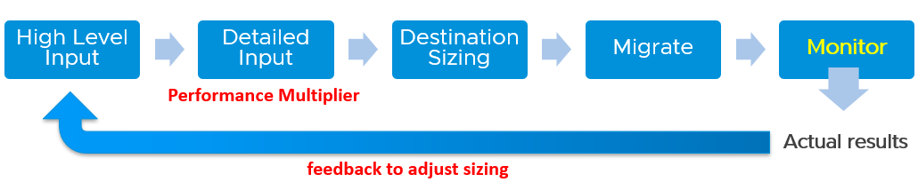
In complex migration, it does not begin with what you to migrate. It begins with the destination. You plan your end state first, add what you want to migrate, and then work back and forth between the 2 sides.

The reasons why you go back and forth are:

| Speed | See Performance Multiplier |

|:---|----|

| Time | In a large-scale migration, it can take months. During that time, the workload may change. The new features added by the application team may alter your sizing |

| New workload | Because the migration period stretches over time, you get new VMs that do not exist in the old clusters. |

| Selection | You typically do not migrate everything and you may use the migration as opportunity to regroup. For example, you may move from per department to per class of service, as your IT business changes from System Builder to Service Provider. |

Migration Group

What happens when your consolidation is not One to One, but Many to Many?

For example, you are consolidating from 47 clusters to 19, but the VMs in a single source cluster will end up in multiple destination clusters. The following examples shows 5 old clusters being consolidated into 3 new clusters. However, the VMs are being reclassified.

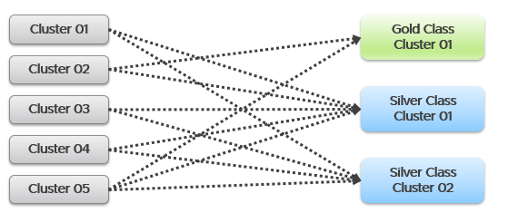
This is more challenging as each VM can potentially have its own usage pattern.

Take for example, you have 500 VM in a cluster, but you only need to migrate 100 of them.

Do you take the individual utilization one by one, estimate the size for that VM, repeat for each VM, and finally simply sum all the VMs up?

You can’t do that as they may peak at different time.

This makes the sizing process cumbersome as you must create group. 1 group for each destination cluster. If you have 30 destination clusters, you need 30 groups. This migration groups become a central piece of your migration monitoring and sizing. They form a pair of “Before” and “After”. The group should consist of just VMs because that’s what you’re migrating. As a bonus, these groups help you in tracking and adjusting later on in the project. As you migrate a VM, remove it from this group.

The main limitation of the migration group is it has no historical data. The data starts from the time the group is created. To see the past, use super metric preview as a workaround.

Rolling Up

As part your overall planning, you need a total number. How do you prevent this number from being inaccurate?

The answer is you cannot.

Take for example, 2 clusters. They have highly cyclical workload, which goes up to 90% and down to 10%. Their workload pattern happens to be complimentary. When Cluster 1 is highly utilized, Cluster 2 is lowly utilization. If you combine them, you get a flat line utilization.

Each cluster has 10 hosts. But because their workload do not overlap, when you combine, the total utilization is only 11 hosts, not 20 hosts.

So what is your sizing requirement at vCenter level?

11 hosts or 20 hosts?

The answer depends on whether you plan to combine them or not in the destination cluster. That’s why you need to begin with the end in mind. If you plan to combine, the answer is 11. If not, the answer is 20. Big difference.

What if you do not know yet?

That means you have 2 numbers, serving as rough estimate of the minimum and maximum.

Use these numbers as the guide. As you migrate, you adjust your sizing.

Reporting

When you are migrating your customers workload to another infrastructure, the onus is on you to prove that you are not causing problems to the VMs or Applications. This is especially true if it’s your idea to migrate, and you are not giving them a choice.

To you as infrastructure team, the migration is a capacity exercise. To your customer the application team, they care more about their VM availability, performance and security. This means you need to quantify the “Before” and “After” to avoid misunderstanding at the VM level. If you have 1000 VM, you need to do 1000 comparisons.

This comparison cannot be done immediately after a VM is migrated. It needs to consider a longer timeline, such as 1 week, for a more complete comparison.

On the other hand, you do not and cannot make the post-migration comparison too long. Compare 3 months of before against 1 week of after.

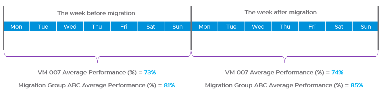
How do you report that the migration does not result in availability, performance and security degradation? If you promise improvement, how do you quantify that?

Consumption

First, you prove that the VM is not doing less work. That means CPU utilization, Disk IOPS and Network Throughput. Expect the numbers not to drop. We cannot combine these counters as they can’t be standardized into 0 – 100%. Why is memory not included? Memory is basically disk space and it’s a form of cache. The memory counter at VM level is irrelevant, and the memory counter at Guest OS level is not within your control.

Contention

Second, you prove that your IaaS is serving the VM well. That means CPU Ready, Memory Contention, Disk Latency and Network Dropped Transmitted Packet. Plot the contention number using the 20-second peak counter. Expect the numbers to drop. If it increases, it remains below the promised SLA. If you are responsible for the Guest OS, then you need to show that queues are not higher post migration. This is why I recommend to keep the VM size. Let the oversized VM be migrated as it is, and right-size it after migration is signed off.

Once you have the above numbers, it’s a matter of plotting them over time.

The above solves it for 1 VM. How to measure for many VMs?

As usual, you create a group to help manage at scale. For each migration batch, you create 1 group. So if you plan to migrate over 35 windows, you have to create 35 groups.

1 migration window should be kept within the day. This makes your Before vs After comparison easier. If you’re migrating 3x on Friday night, Saturday night and Sunday night, then it’s 3 migration windows.