Capacity

Part 2 Chapter 5

The capacity dashboards aims to implement the capacity concept covered in Capacity Management chapter, and complement the existing product pages.

Overall Design

You may notice that the performance dashboards and the capacity dashboards share similar layout. The reason is there is commonality in both pillars of operations.

The suite of dashboards work together as one integrated set. They also have similar design.

Goals	Determine overall capacity. Cover compute, storage and network. Network covers ESXi physical NIC, NSX Edge and NSX Manager.
	Optimize capacity. Reclaim, rightsize, and redistribute.
Questions	Examples of questions answered by the dashboards:
	What’s the overall capacity? Do we have enough CPU, memory, disk and network to meet present demand + demand in the near future?
	Any hot spot? Do we need to rebalance?
	How severe is the wastage? How much can we easily claim within a month? How much will take much longer to reclaim?
Assumptions	Users will use the built-in pages. These dashboards are designed to complement, not replace.
Target Users	Capacity Team. This is the main target. The team responsible for overall capacity life cycle, from planning to upgrade. Not interested in day to day, such as a host goes down or put into maintenance. Keen on long term and top down view, as they are planning future expansion and ageing hardware technological refresh. Their primary focus is the Provider
	Operations Team. The team running the day to day, live operations. Not interested in long term, both the past and the future. Their primary focus is the Consumer, especially oversized VM.
	Storage Team. Specialist team. Collaboration become critical if the architecture is “thin on thin”.
Usage frequency	Weekly
	Quarterly
Features	The dashboard is designed “top down”. It has 2 sections: summary and detail. The summary lets you see the big picture. The detail section is placed below the summary section. It lets you drill down into a specific object. For example, if it’s a VM capacity, you can get the detail capacity of a specific VM.
	Quick context switch. You can cycle through objects quickly without changing screens or opening multiple browser windows.
	UI wise, the dashboard uses progressive disclosure to minimize information overload and ensure the webpage loads fast. On the other hand, so long your browser session remains, it remembers your last selection
	Color coded. A high capacity remaining could indicate wastage. For ease of identifying, wastage is shown by a new color. Dark grey indicates wastage as capacity is not used. In fact, there can be performance problem is the low utilization was caused by bottleneck somewhere else
	Complement the out of the box pages by visualizing information differently and giving more choice of customization. For examples, the reclamation size is grouped into buckets so you can focus on the largest reclamation opportunities first, and trend charts are provided so you can quickly see the growth over time, without changing context (e.g. open a new screen).

There are 2 types of capacity management

• Consumer. You focus on a single VM, container or application. You want to right size them and reclaim unused portion.

• Provider. You focus on the shared infrastructure as the problems impact many consumers.

For cluster, special types of cluster alter the capacity model. One example is stretched cluster. It needs its own capacity model and visualization. You will need to have an object or custom group for each site, and then displays them side by side.

Compute Capacity

The compute capacity dashboard covers vSphere clusters with their associated ESXi host and resource pools, as they impact the cluster capacity.

The dashboard is designed for cluster, and not standalone ESXi host. The layout has these sections:

• Multi Clusters. It should have a table listing all clusters.

• 1 Cluster. What’s the overall utilization. It should show both CPU, memory, and network.

• Subcluster. Break into the ESXi hosts. This is only needed if there are imbalances.

Overall Analyzis

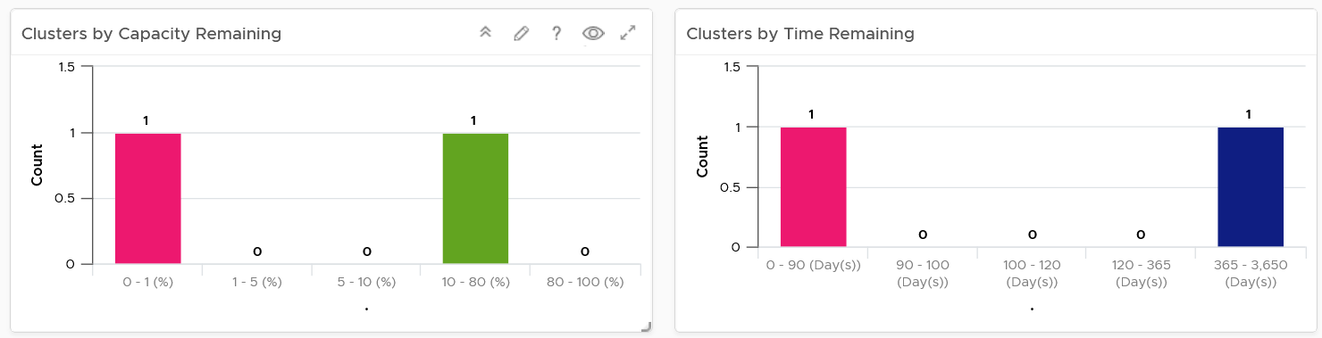
The 3 bar charts show all the clusters, summarizing the overall situation. The first 2 are shown below.

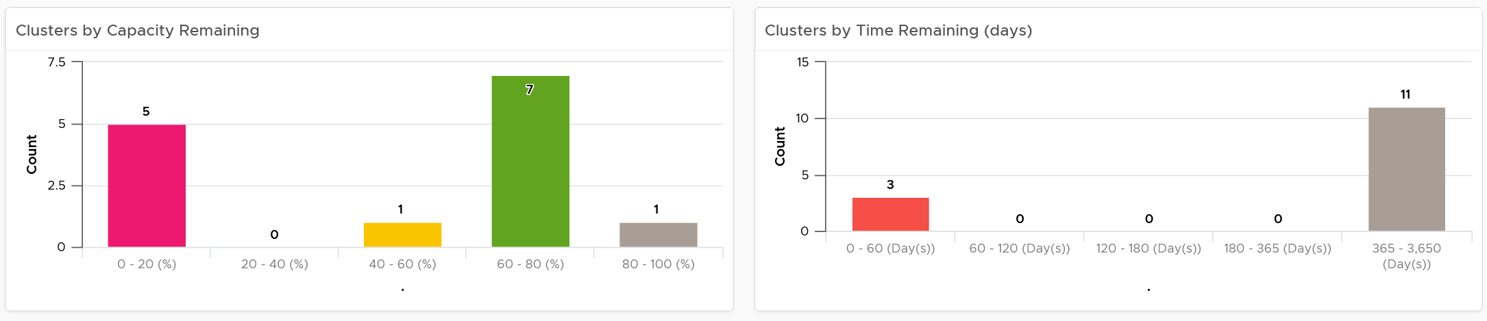
The first two bar charts work together. Just because you are running low on capacity does not mean you are running out of time. Cluster with a cyclical load that hits high utilization but never trends toward 100% will have low capacity remaining, but plenty of time remaining.

Generally speaking, the ideal situation is low Capacity Remaining and high Time Remaining. This means your resources are cost effective and working as expected. For clusters where you intentionally need to run at low utilization (e.g. stretched cluster), increase its buffer accordingly so the capacity metrics will reflect that.

The 3^rd bar chart is VM Remaining. It gives more complete contexts, as different clusters can have different VM size.

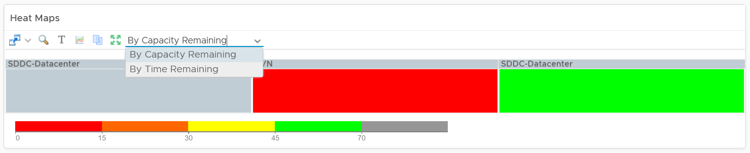
The bar charts can’t show the parent data centers. It also can’t show all the clusters, individually. For a large environment, a heat map comes in handy.

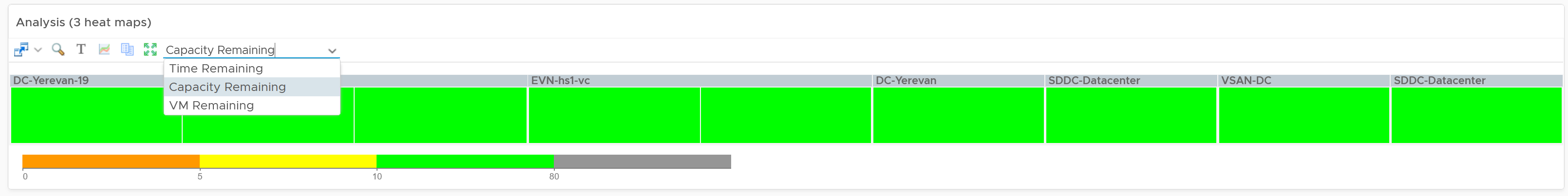
The three heat maps are Time Remaining, Capacity Remaining, and VM Remaining.

The color indicates usage. Low utilization is marked as grey, not green, as it represents waste.

Why is the box size made identical?

For ease of use and better focus on the action to be taken. Otherwise the small clusters will be dwarfed by the large ones.

If your cluster sizes are not standardized, create another heat map, and use the number of ESXi hosts to show the size difference.

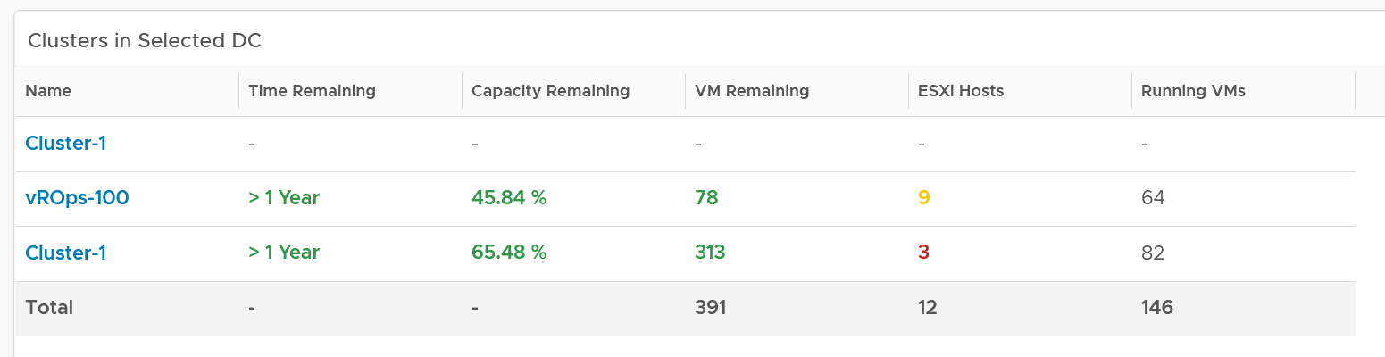
A table provides the next level of details.

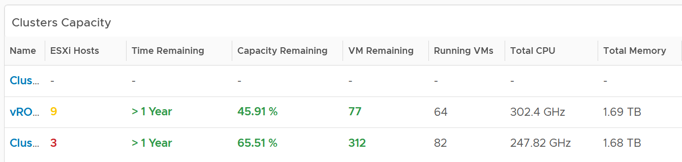
The number of ESXi hosts are color coded as smaller clusters have relatively higher overhead.

Cluster Analyzis

Select a cluster from the table. Its detail capacity will be automatically shown.

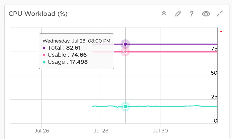
Performance

The first thing it shows is the cluster performance. Make sure this is within your expectation.

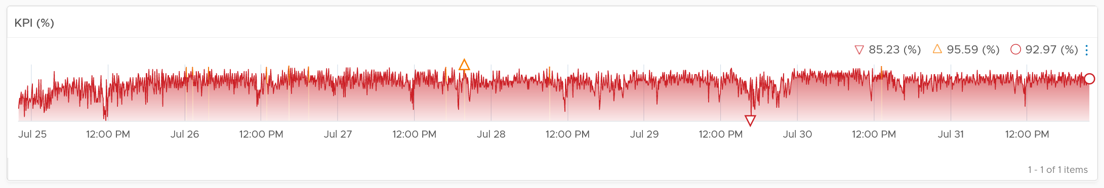
The counter is covered in Performance chapter and Performance dashboard.

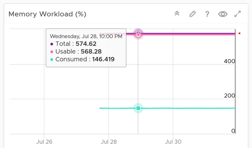
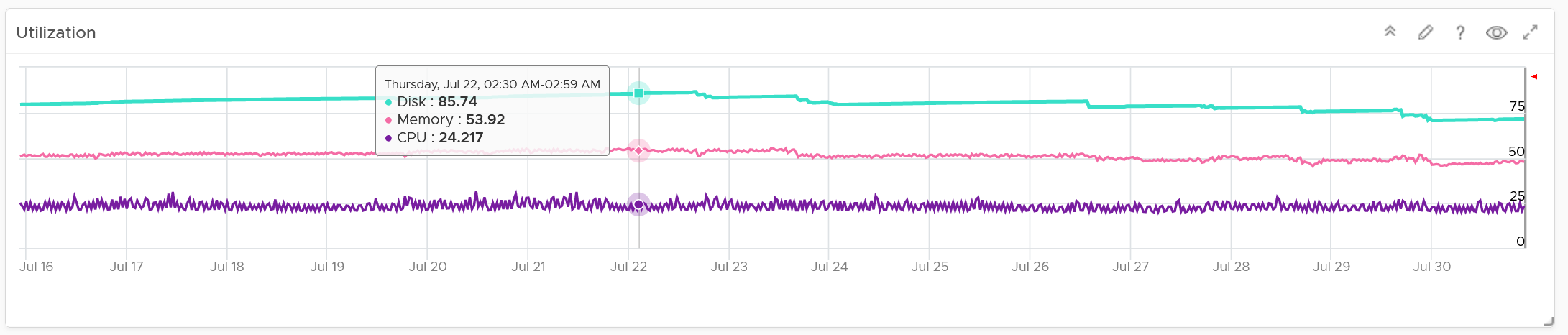
Utilization

The next chart is utilization. It’s showing in %, as it’s relative to your usable capacity.

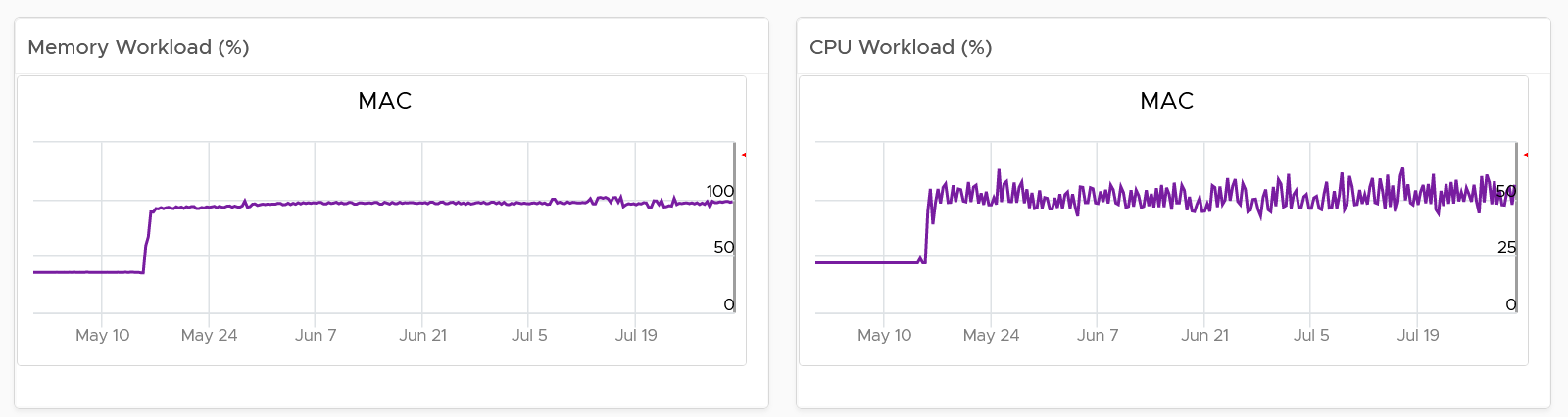
Utilization displayed for three months and not one week. The daily average is displayed and not the hourly average, so you can focus on the overall trend.

For memory, the focus is on consumed memory and not active memory.

If it’s useful to you, add peak to complement average utilization. The peak is defined as the highest among any ESXi hosts. If the peak is higher than the cluster-wide average, then the cluster is imbalance. Find out the cause of imbalance and optimize it.

If you have the screen real estate, add the absolute utilization.

Allocation

Next is Allocation, as not all demand is real. You need to use both models.

Workload can be low, but is overcommit ratio high? Newly provisioned VMs tend to be idle for weeks, and suddenly grow.

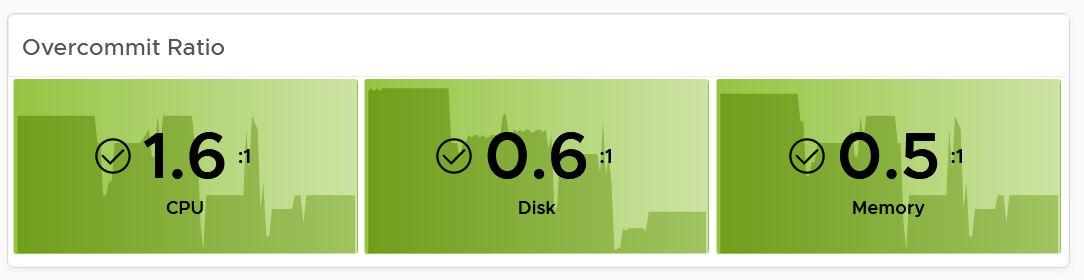
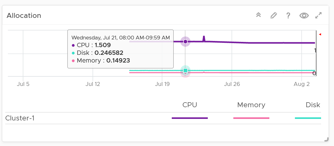
You can see the trend of the 3 components together on a chart if that is relevant to you. In general, your CPU overcommit should be the highest, followed by disk (due to thin provision). Memory overcommit tends to be near 1 due to its nature as cache.

Use the line chart to see the trend. As usual, the data is averaged hourly so you can focus on the big picture.

Next is the VM Count. A trend line of number of VM over time is important to spot if there are many newly provisioned VM. If you see VM growing but demand remains low, that's a sign of potential demand coming up in the future.

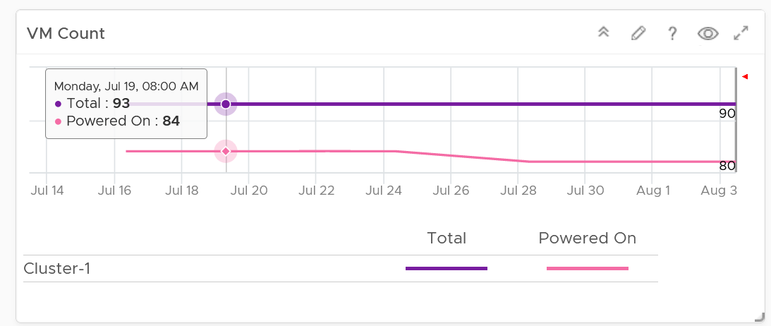
BTW, the overall VM:ESXi ratio is a common number cited to senior management. It’s often measured as cost efficiency proof.

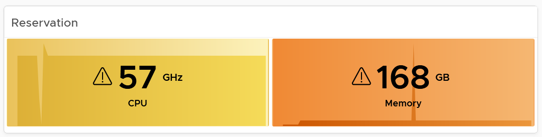
Reservation

Reservation can impact the efficiency of your cluster. Why is the cluster low on capacity? Is it because of real workload, or just reservation?

If your cluster size varies, complement the reservation number by showing relative value. Once you have a standardized number, you can visualize them on a heat map! This enhancement requires super metric, good practice! 😊

Reclamation

As covered in the Capacity Management chapter, there are 6 types of reclamation. Some of them are shown below.

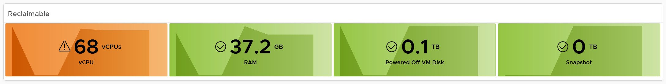
If it’s relevant to your environment, add the number of undersized CPU and undersized memory.

ESXi Analyzis

Just because the cluster capacity is good, does not mean there is no issue at ESXi level. Imbalance is common issue, especially in large cluster and stretched cluster.

The following table shows all the member ESXi. You can see the imbalance clearly, thanks to the color code.

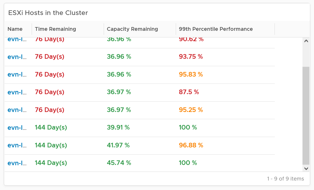
The 99^th percentile Performance column takes the 99^th percentile value of the ESXi Performance (%) metric. The reason we’re not taking the worst performance (which is equivalent to 100^thpercentile) is to rule out outlier. In addition, the performance threshold has been set to be stringent.

Select one of the ESXi. All its detail will be automatically shown.

Both CPU and memory trend line charts show if it’s steady demand, cyclical demand, rising demand, or declining demand. The trend is as important as the present value. To see trend, you need to see over longer time. Utilization is displayed for three months and not one week. The daily average is displayed and not the hourly average and the focus is on memory consumed and not memory active. Note that memory consumed includes the total memory consumed, so it includes memory consumed by VMkernel.

Both total and usable utilization in terms of memory and CPU are displayed. This gives you the absolute amount of capacity.

A technology refresh is often used to address capacity shortage. The relevant configuration shows the hardware model and specification to help you determine the age of the hardware.

VM Analyzis

What’s causing the low capacity remaining? Which VMs are impacting what infrastructure resource (CPU, memory, disk space)?

Use the following table to analyze. It lists either the VMs in the cluster or host.

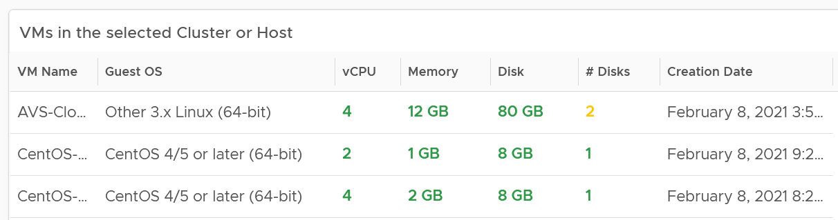
You can select one of the VM, and additional relevant information will be shown.

You can enhance this by using 2 heat maps, one for CPU and one for memory. Shows all the VM, sized by configured and color by capacity remaining. If you see many large VMs running low on capacity, that means you should stop provisioning until you upsize existing VMs first.

Datastore Capacity

This dashboard complements out of the box capacity pages and dashboard. It focuses on storage, provides overall picture, and highlights the datastores that need attention. ​

Overall Analyzis

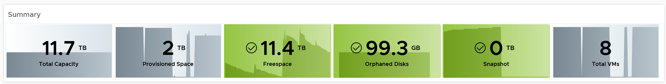
“What do I have in terms of capacity?”

The summary banner answer basic questions like this.

If required, customize it. I keep it simple as you don’t actually have 1 contiguous storage pool. Just because you have 100 TB available in South Pole DC does not mean your servers in North Pole DC can use it, unless you tunnel dark fibre over earth core.

Next is the distribution chart. Do they look familiar?

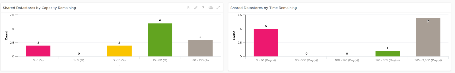
It’s intentionally designed to be consistent with the Cluster Capacity dashboard.

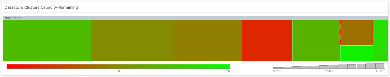
As you can expect by now, next in the dashboard is the heat map.

There are three heat maps, the primary being Remaining Capacity heat map. The 2 other heat maps cover Used Capacity. One of them is designed for environment that use Datastore Clusters.

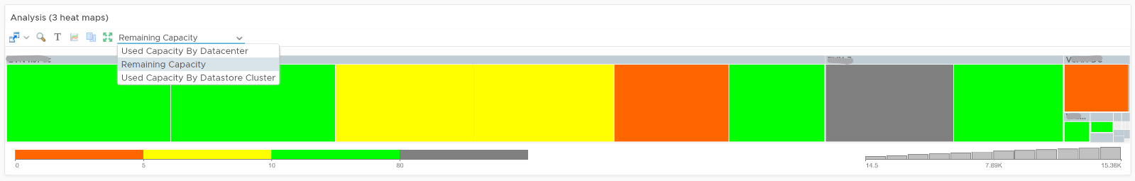
Each box represents a datastore. If you have many datastores, the heat map will group them. You can drill down to see its members. The larger the datastore, the larger its box is. If you have many small datastores, consolidation can make operations easier.

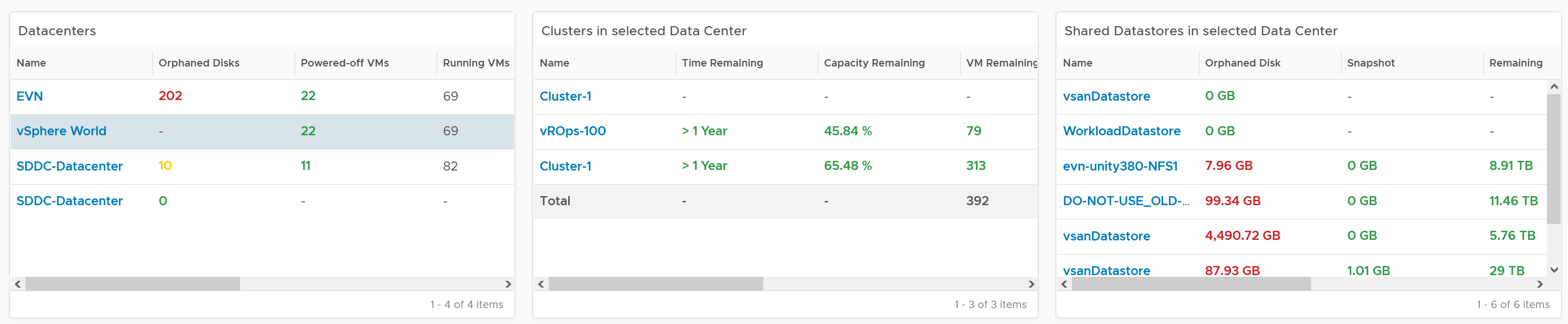
Following the design used in Capacity dashboard, next is the table listing all the Shared Datastores.

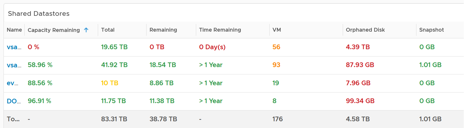
The table provides a summary, showing all datastores a glance. They are grouped by Data center. If you use Datastore Cluster as your standard and it suits you better, replace the grouping with it.

By default, the table is sorted by the least capacity remaining.

There are 3 reclamation opportunities: powered off VM, snapshot, and orphaned VMDK.

Why is Idle VM not included?

Because you should power off first, and let it go through powered off period before deletion.

Datastore Analyzis

Select a datastore from the table. Its detail capacity will be automatically shown.

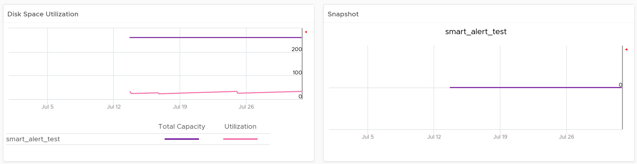
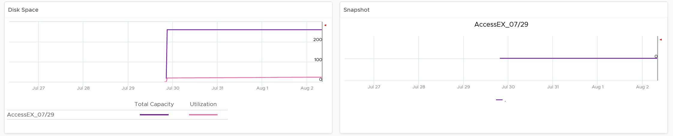
The snapshot should be 0 GB. If it is not 0, then it should be temporary. A snapshot lasting beyond a few days should be investigated.

Orphaned Disks are VMDK files that are not associated to any VM. Expect it to be 0.

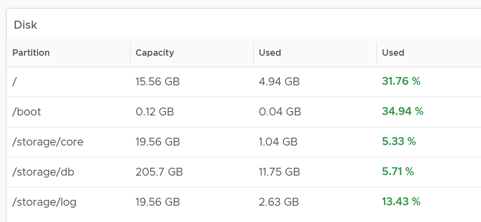
For disk space, the total capacity, allocated and actual used are shown. What does it mean when the provisioned disk space metric grow but the actual used does not?

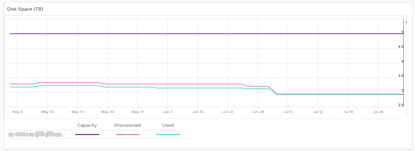
That means the VMs are yet to use it. Watch out, you can run out of space sooner than expected.

The value is daily averaged to show the big picture. Having 5-minute spike can visually make the chart harder to read.

If you use allocation model, add a second line chart showing the allocation over time. Add a threshold so you know how close you are.

VM Analyzis

If you need to analyze at VM level, review the table listing all the VMs in the datastore.

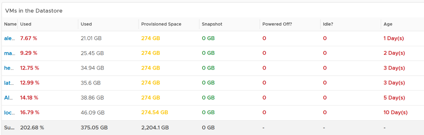
If you have hundreds of VMs, create a heat map showing all the VMs. Color it by the used space so you know if the VM is reaching its full size. Size it by the allocated size so you can see who the big VMs are. If the big VMs have plenty of space to grow, watch out.

Click on the VM you want to investigate further. You get to see its usage over time.

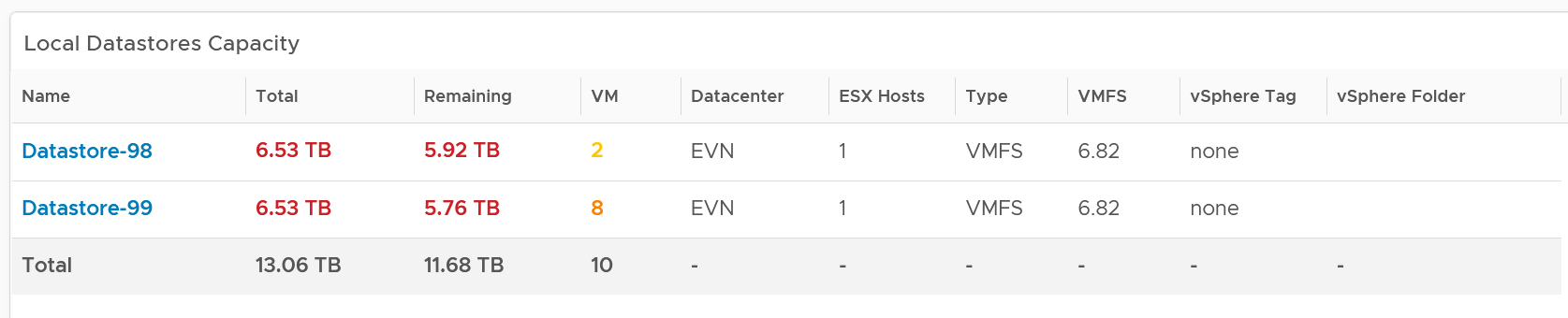
Local Datastores

They are shown separately as a table on its own, at the end of this dashboard. Avoid running VMs on local datastores, unless its storage requirements can be met with a local disk and it does not need vmotion.

Points to Note

If you are using “thin on thin”, meaning the underlying LUN is also thin provisioned, add visibility into the physical array.

The dashboard does not have datastore clusters. If your environment use it, modify this dashboard or create a new one. In a large environment with many datastores and datastore clusters, add a View List to list the datastore clusters so you get summary information. From this list, drives the datastore view list. Alternatively, create a heat map, listing the datastore clusters.

­vSAN Capacity

The vSAN Capacity dashboard complements the vSphere Cluster Capacity dashboard by showing vSAN related capacity. It focuses on the storage and vSAN specific metrics, and does not repeat what’s already covered. That’s a long winded way to say you gotta use both dashboards to manage vSAN capacity 😊

Because the metrics are vSAN specific, this dashboard does not list non vSAN cluster.

Overall Analyzis

The dashboard starts with the familiar bar-chart combo that Cluster Capacity dashboard has. The difference is this focuses on the vSAN disk space, not compute and network.

Similar to Cluster Capacity dashboard, next is a heat map. There are 2 heat maps provided.

Why is the box size made identical?

Head to the Cluster Capacity dashboard for the explanation.

As you can expect, a table provides the next level of details. The difference is you get vSAN specific metrics.

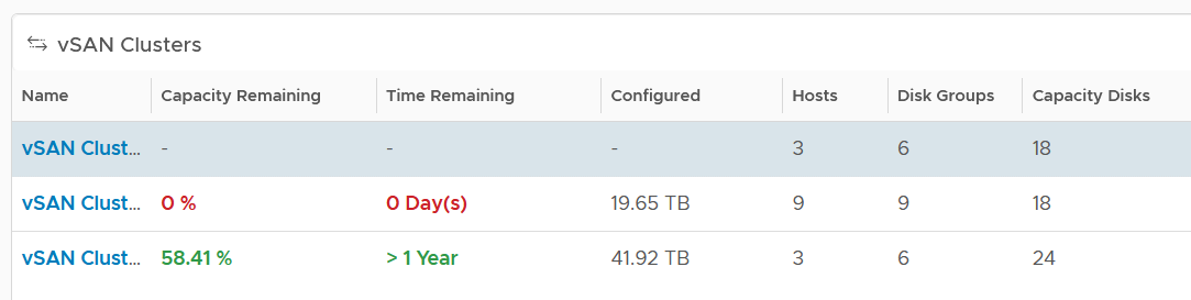
If it’s useful, add metrics such as total disk capacity and used.

Cluster Analyzis

Select a vSAN cluster from the table. Its detail capacity will be automatically shown.

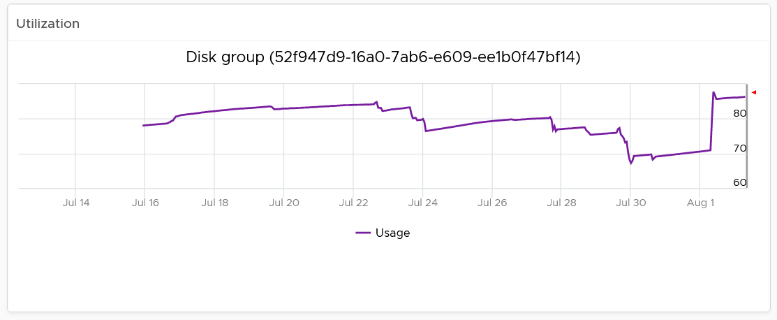
Utilization

It’s showing the utilization for all 3 elements, as you need to consider all three. Network is not shown as typically it’s not an issue and it’s complex to model.

Just like physical array, there can be hot spot and imbalance. The following heat map shows individual disk groups.

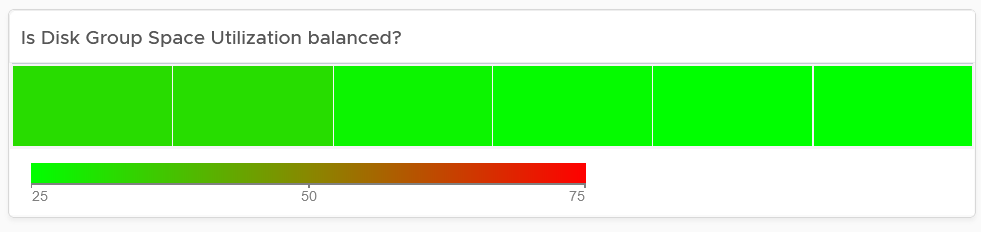
Notice they are all green but not identical. It’s normal for them to have minor variance.

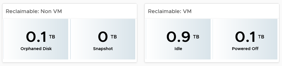
Reclaimable

It’s a key component of proactive capacity management. The dashboard shows you both the VMs and non VMs portion.

Dedupe and Compressed

The scoreboard shows details on this area.

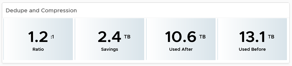
If you are concerned with the CPU usage from the dedupe and compress feature, add a line chart of vSAN CPU usage.

Disk Group Analyzis

If there is imbalance, you can drill down into each disk group. Otherwise, skip this section.

The following table shows all the disk groups in the cluster. Their usage may not be similar but they should not deviate drastically.

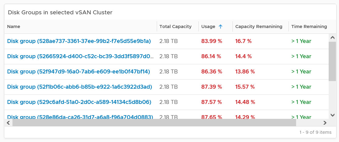
To see any of the disk group usage trend, click on it.

In addition a heat map is provided to see the usage among the capacity disks in the selected disk group. Expect them to be uniformed at this level as it’s RAID striping.

VM Analyzis

You can get down to individual VMs in the selected cluster, and check their usage and snapshot.

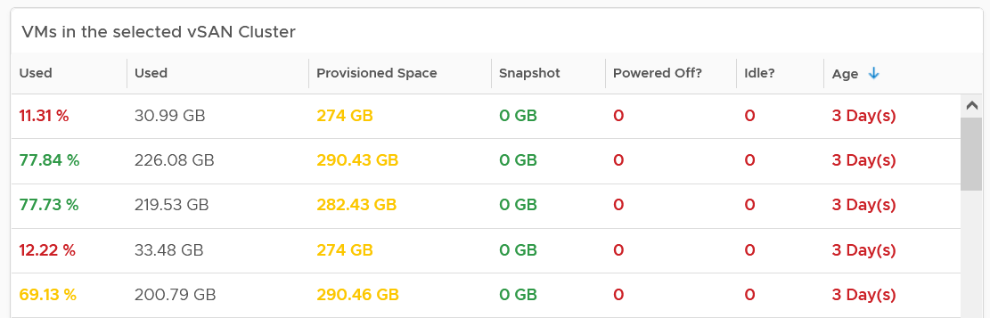
To see the usage trend, select the VM.

In addition, the relevant configuration of the selected VM is also shown.

VM Capacity

The dashboard helps you analyze the capacity of all the VMs, with ability to drill down into each VM.

Overall Analyzis

The dashboard begins with a table listing all your data centers.

vSphere World is also included so you can see all the VMs from all data centers. Unlike infrastructure objects, there are potentially tens of thousands of VM. So take note that the charts will take longer due to refresh if you select vSphere World.

How do the following 2 charts provide insight into the capacity of all the VMs in your environment? What’s the ideal distribution?

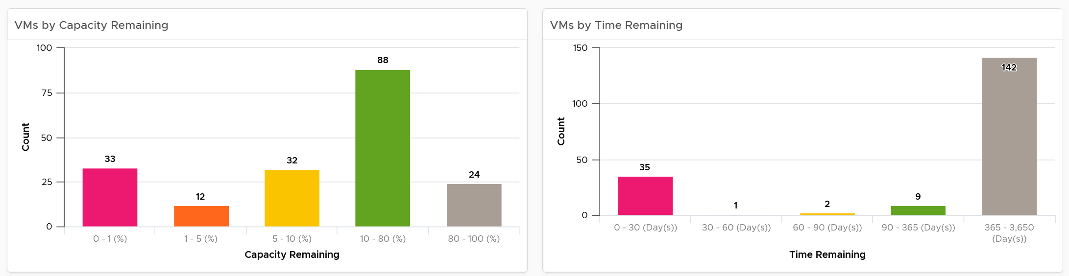
The first chart groups them by capacity remaining, while the second one by time remaining. Ideally, you want all of them to be low on capacity remaining (meaning the given capacity is actually fully used) but high on time remaining (meaning they do not need additional).

The bucket size has been designed to map the default settings in VM capacity policy. If you change it, also change the value in policy so it’s consistent.

The heat map provides additional view by grouping them by cluster. It helps you spot which cluster is at risk (majority of its VMs need more capacity) and which cluster can provide extra resource (majority of its VMs are not using their capacity).

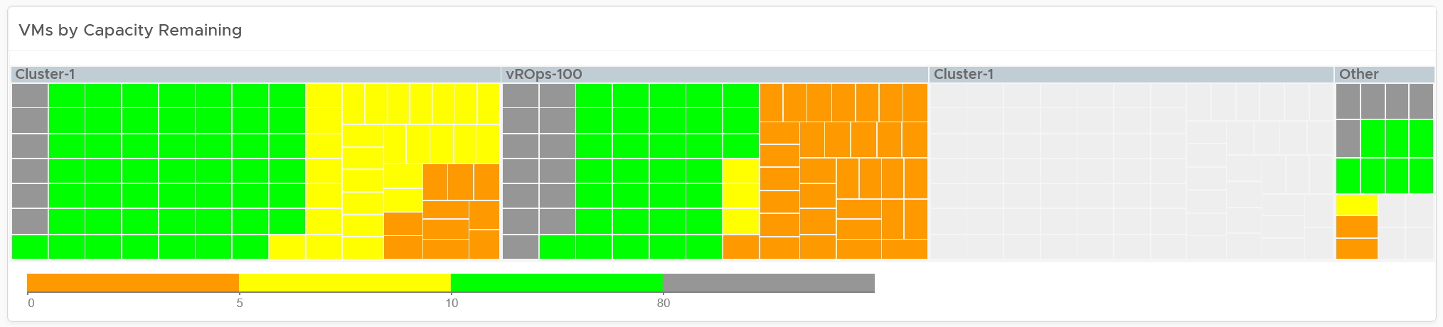
Review the heat map. It provides the next level of details by grouping the VMs by clusters, so you can see which clusters need attention.

Note the VM size has been standardized for better visualization. If it suits your capacity team better, add the size. Note that by doing that you have to pick CPU or Memory, so you may have to create 2 heat maps.

Review the table listing all VMs in the selected data center.

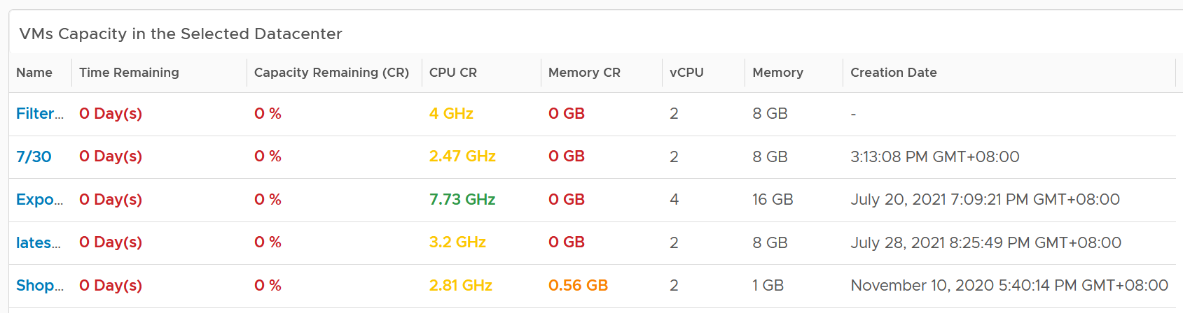
The list is sorted by the VM with the least capacity remaining. If sorting by Time Remaining suits your operations better, modify the dashboard.

The table is also color coded. Take note that the threshold is unable to show the grey (wastage) color.

The creation date is added for the same reason in idle VM case.

VM Analyzis

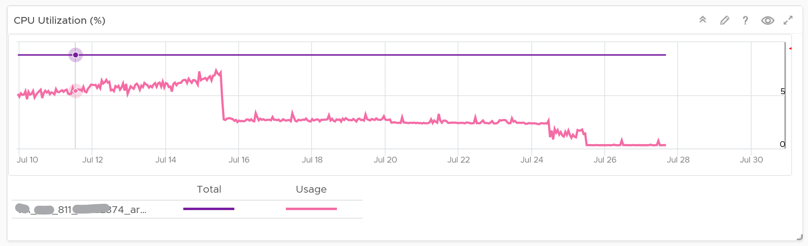
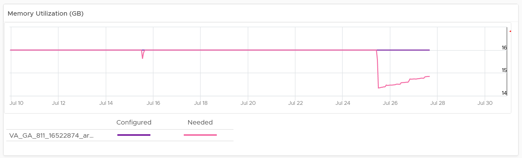
Select a VM from the table. Its detail capacity will be automatically shown.

You get both the CPU and memory trend over time. 3 months data is shown, and they are averaged to hourly so you can see the overall trend instead of spiky chart.

For memory, it uses Guest OS, for the same reason explained in VM Rightsizing dashboard.

For the disk, it uses the Guest OS partition. Do not use VM virtual disk as there may not be 1:1 mapping to the actual partition.

Right-sizing recommendation is also shown for both CPU and Memory. Unlike physical server, it's important to right-size VM for the benefits listed here.

For CPU, the CPU Usage counter is used instead of Demand. Use the knowledge you learned here to figure out why.

For disk, it’s showing at the Guest OS partition level. There is no overall capacity at VM level because different partitions have different capacity.

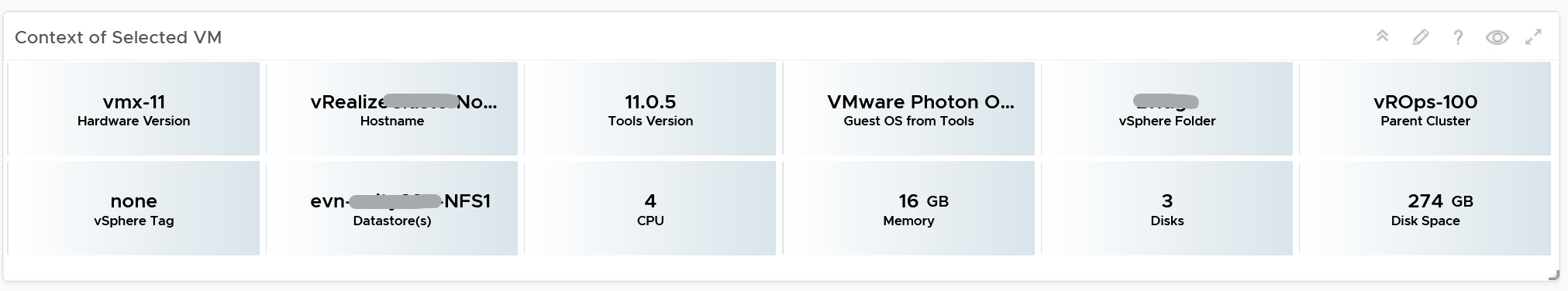
Relevant Configuration

The relevant configuration is automatically shown to give context to the VM.

Information such as VM Owner and business units can be useful in the analyzis.

Reclamation

The Reclamation dashboard helps you managing various types of reclamation that can be done on VMs and datastore. It is designed for both the Capacity team and the Operations team.

Overall Analyzis

The scoreboard provides a summary of the total reclamation. Guest what infrastructure resource is missing from the scoreboard?

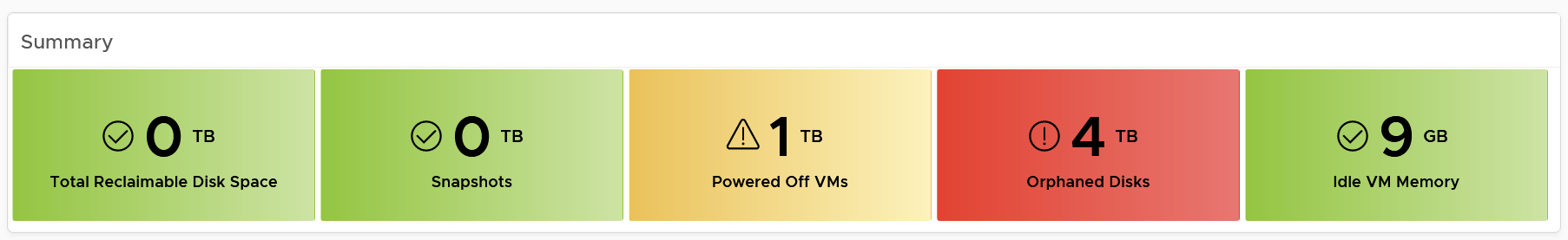
CPU is missing. Because you’re reclaiming blank air.

You can drill down at either Data Center level, cluster level or datastore level. Datastore level is required as orphaned disk does not have VM association, hence it’s not related to any cluster.

The table above can drive all the charts underneath them, shown below, giving you a flexible way to slice the information. Take note that the datastore table only drives the snapshot table. The reason is traversal spec. The view widget can only use 1 traversal spec.

The summary information will be automatically shown. To show from all clusters, select vSphere World. This object covers all clusters. Take note that the charts will take longer due to refresh due to higher amount of data.

If necessary, adjust the bucket size in the charts to suit your operational requirements.

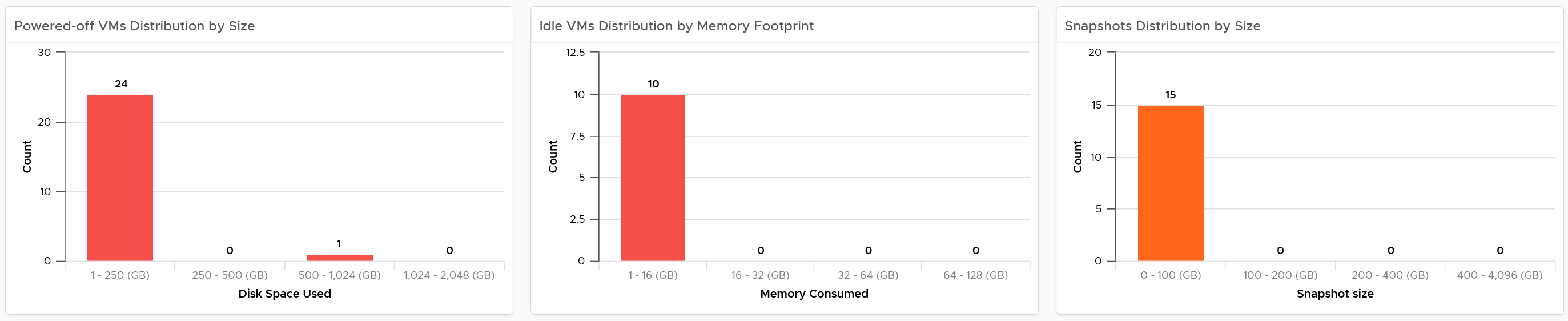
The reclamation potentials are presented as 3 bar charts, each corresponds to an area you can reclaim:

• Powered off VMs that are no longer needed contribute to wasted disk usage. Consider deleting them to free up space or moving them to archival storage.

• Idle VMs are running, but not being used actively. These VMs consume memory that may be used by active VMs. Consider removing these VMs to reduce memory contention. Guess why is VM-level metric used instead of Guest OS metric?\

  Memory reclamation is based on the memory footprint at the parent ESXi. The value inside the Guest is not what is being reclaimed, and so it is irrelevant

• Snapshots are meant to be temporary and can cause performance issues and waste disk space if not deleted after a few days.

Focus on snapshot first, as it does not involve changing VM.

Next is powered off VM. The longer it has been powered off, the lower the risk of deletion. Ideally, you want a confirmation from the owner, and have a back up outside vSphere. This is why it’s important to have meta tag such as VM Owner email address. Note if the VM has snapshot, it’s included in the calculation, so there can be double counting since the VM also appears in the snapshot table.

Idle VM

As the VM is still running, it’s relatively harder to reclaim as shutting it down may require approval from the VM Owner.

BTW, if there is nothing to reclaim, you get a blank table. The following example shows no VM meets the criteria for either powered off or idle. If you suspect the table is wrong, review your criteria.

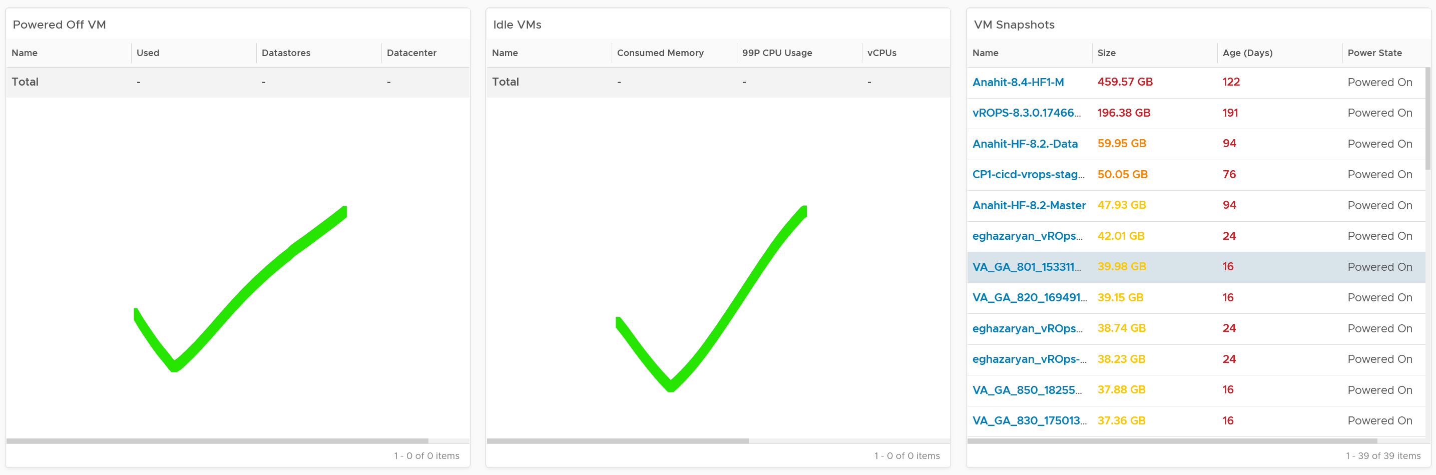
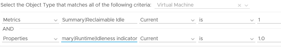
We discussed in Capacity chapter that both metrics need to be true to ensure the list does not contain VMs that has recently become active.

Let’s drill down into idle VM as that’s the most complex part. Guess why we show the 99^th percentile CPU usage?

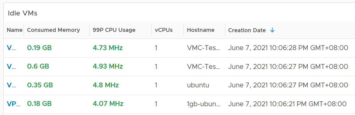
The 99P CPU Usage shows the CPU usage at 99^th percentile during the time period. It’s a handy way to check if it’s indeed idle. Essentially, if it the CPU utilization is low for 99% of the time, the VM could indeed be idle.

Why is the Creation Date especially important for Idle VM case?

The answer is newly provisioned VM may remain unused for months. The following show how to set it.

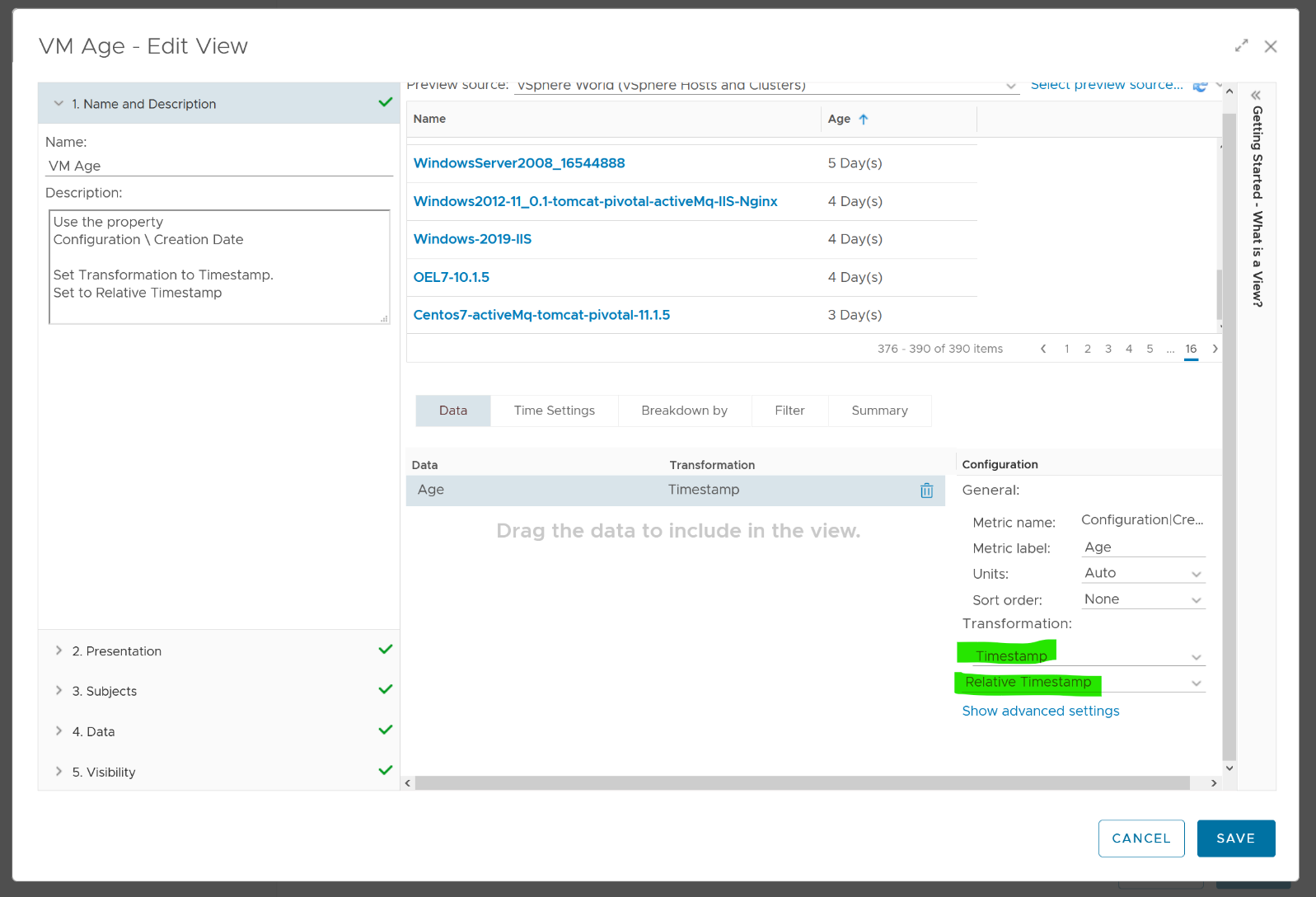
Choose VM property Configuration \ Creation Date, then choose the Transformation: Timestamp and then Relative Timestamp.

VM Analyzis

To analyze VMs for reclamation opportunities, select a VM from one of the three tables (Powered Off VM, Idle VMs or VM Snapshots). Its detail value over time will be automatically shown. Notice the VM name is the same in all the 3 charts.

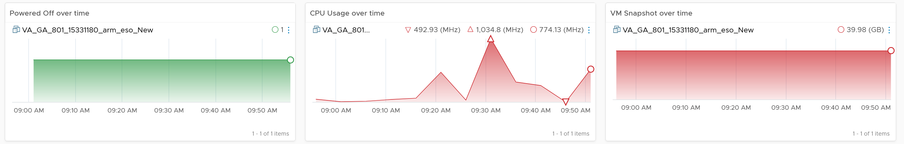
Powered off over time shows VM status (on/off) over time. 1 = true, meaning the machine is powered on.

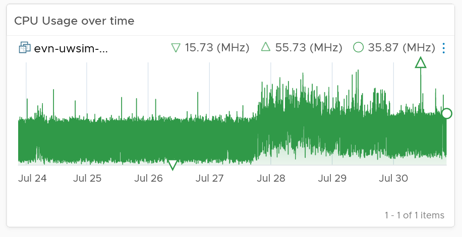
CPU Usage over time provides insights into the aggregate CPU usage, including peak usage periods. This way you can validate that an idle VM has not had any brief usage. What you want to see is green over a long period of time, as shown in the following example.

If the snapshot is expanding rapidly, ensure that the VM disk is small (relative to size of the underlying datastore) as it can fill up the datastore.

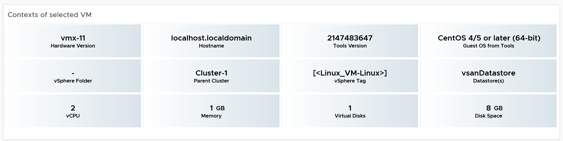
Lastly, the relevant configuration of the VM is also shown to give context.

Points to Note

If your environment is large, change the dashboard filter to a functional filter. Group by the class of services such as gold, silver, and bronze and default the selection to the least critical environment. In this way, you can be more active in reclamation.

If reclaiming is a long drawn manual process in your organization, add a filter by department or VM owners. To organize your reclaim efforts it is helpful to create custom groups to make it easier to filter by department or VM owner. This can make it easier to seek approvals and communicate with anyone who may be impacted.

You should enhance this to include Trim and Unmap. Happy to collaborate and make this into the product. We need to check on only the thin provisioned disk. We should also check at the array level, using the TVS adapter.

Rightsizing

The VM Rightsizing dashboard helps you in adjusting the VM size for best long term performance at lowest cost. It covers both undersized and oversized scenarios. It’s not designed for short term, 5-minute performance burst. The reason is high utilization is actually good for performance. As a result, this dashboard is categorized under Capacity and not performance.

It is designed primarily for Capacity team, not day to day operations team.

Overall Analyzis

The scoreboard provides a summary of the total undersized and oversized CPU and memory.

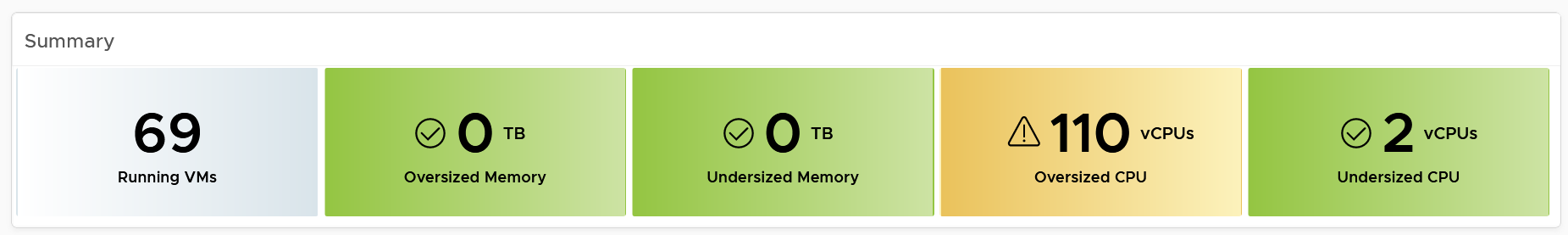
If the number is acceptable to you, that’s it. No need to further analyze.

The reason why I’m not adding the number of VMs that are undersize or oversized is screen real estate. It needs 4 metrics to account for all the combination.

You can drill down at either Data Center level or cluster level. In most cases, rightsizing analyzis should be done at Cluster level as VMs typically do not move inter-cluster. At cluster level, the table looks like the following. Guess why are the cluster capacity metrics shown?

The metrics are shown to give better context. Focus on reclaiming on cluster that is low on capacity remaining. For upsizing VMs, ensure the parent clusters have good capacity remaining.

The distribution charts showing the rightsizing is automatically shown. Let’s dive into the undersized first as it’s more common. Why are the vCPU to add focused on the first 8 vCPU, and memory to add focused on the first 16 GB?

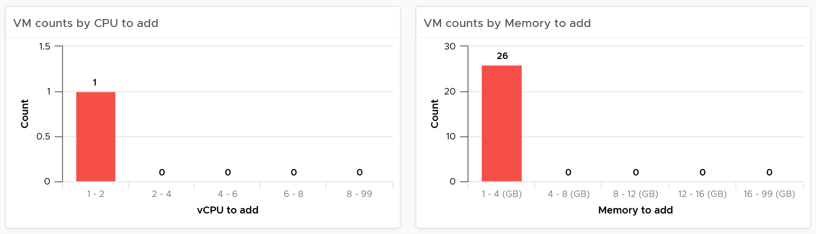
The main reason is you want to avoid adding large amount without strong justification.

For CPU, the primary justification is the CPU run queue counter, not the CPU usage. Even if the CPU Usage is flat out 100%, if the CPU run queue is below 2 per vCPU, you don’t need to add many vCPU.

For memory, Guest OS does not provide deep visibility into the depth of memory shortage. Adding memory may also requires changing application setting so it can take advantage of it.

Do the same capping for oversized VM. To make a drastic reduction, discuss with the VM Owner. Reducing memory may also requires changing application setting, especially application that manage its own memory such as JVM and DB.

Other than the bar charts, you also get the table listing the actual VM. You have 2 tables, one for undersized and one for oversized. Why can’t we just use 1 table?

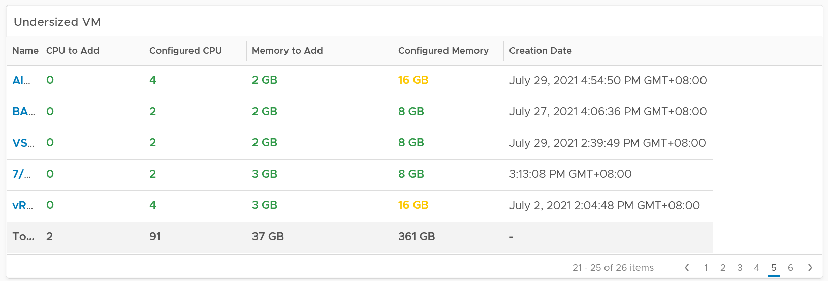
The reason for separate table is the business processes for oversized and undersized VMs are different, as one requires the affected VM to be shut down and the VM Owner to give back resources. For upsize, you want to add incrementally or even automate this process. For downsize, you want to remove in one change window as the effort to reduce is the same and there will be only one downtime.

CPU/Memory to remove is color coded to help you prioritize. Red color means they are excessively oversized.

Configured CPU/Memory is color coded to help you focus on the large VM. They are shown in red.

Take note that a VM can appear in both tables. It can be undersized for CPU, oversized for memory, and vice versa.

Here is the table for oversized.

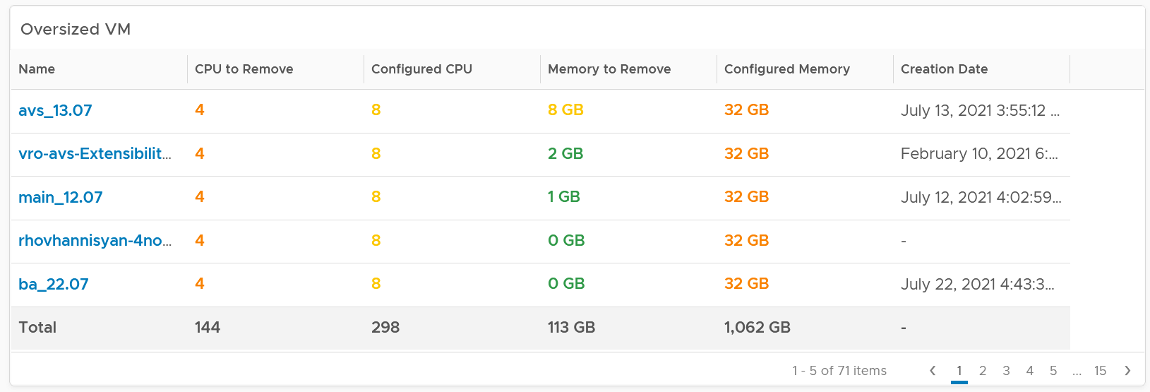
The metrics used are Summary \ Oversized \ Virtual CPUs and Summary \ Undersized \ Virtual CPUs. It stores the capacity engine calculation on recommended number of vCPUs that must be removed or added.

VM Analyzis

Select a VM to investigate further. You get its utilization automatically shown. Naturally, you expect the utilization to go higher if the VM is reduced.

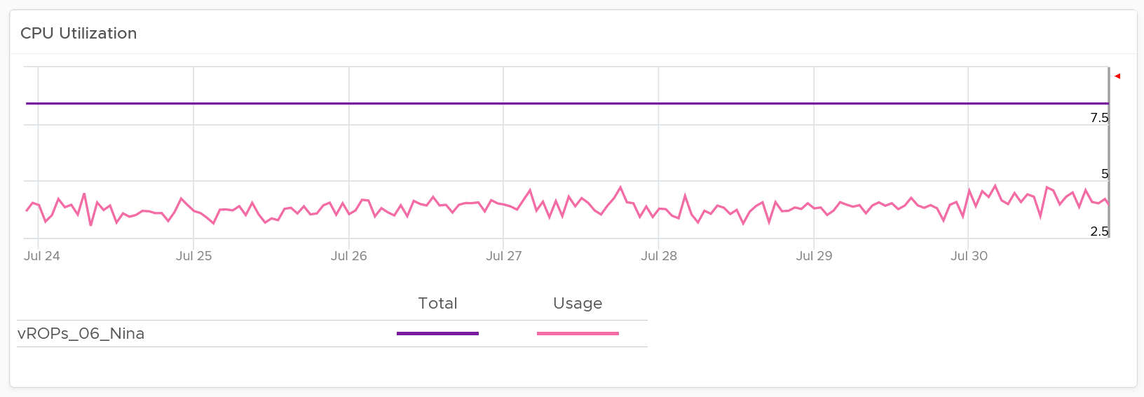
Take note since the purpose here is capacity and not performance, you should not dive into individual vCPU utilization, nor increase collection granularity to shorter than 5 minute (e.g. to 20 second).

Having said that, rightsizing a VM can help improve its performance, or maintain its current performance. How do you prove that?

You show the performance bottlenecks, such as CPU ready and CPU run queue. The following is what you get out of the box.

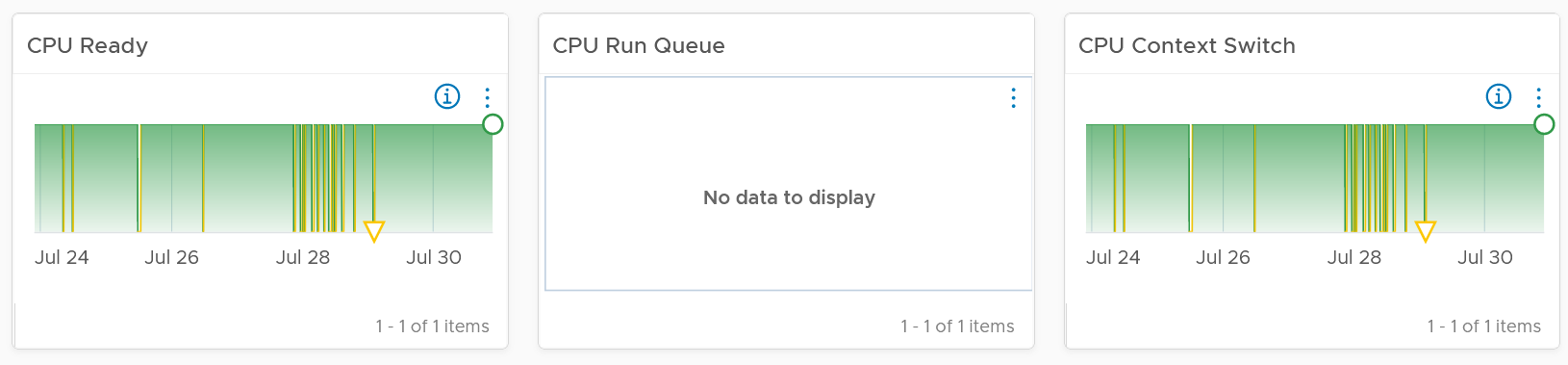
You should expect the VM contention metrics such as CPU Ready and Co-stop to either drop or remain the same.

You should expect the Guest OS CPU Run Queue to remain the same. It might go up a bit, so long it is lower than 3 per vCPU, no need to increase CPU size despite it’s running high. If you want to be safer, modify the widget to use the 20-second counter.

You should expect CPU Context Switch to be less, as there are less CPU to switch. All else being equal, this is a positive change.

If you have the need, add more metrics such as Co-stop.

Memory utilization is collected from the Guest OS. If guest OS metrics are not available, then you will only see the Configured counter. Guess why isn’t there a fall back to VM level memory?

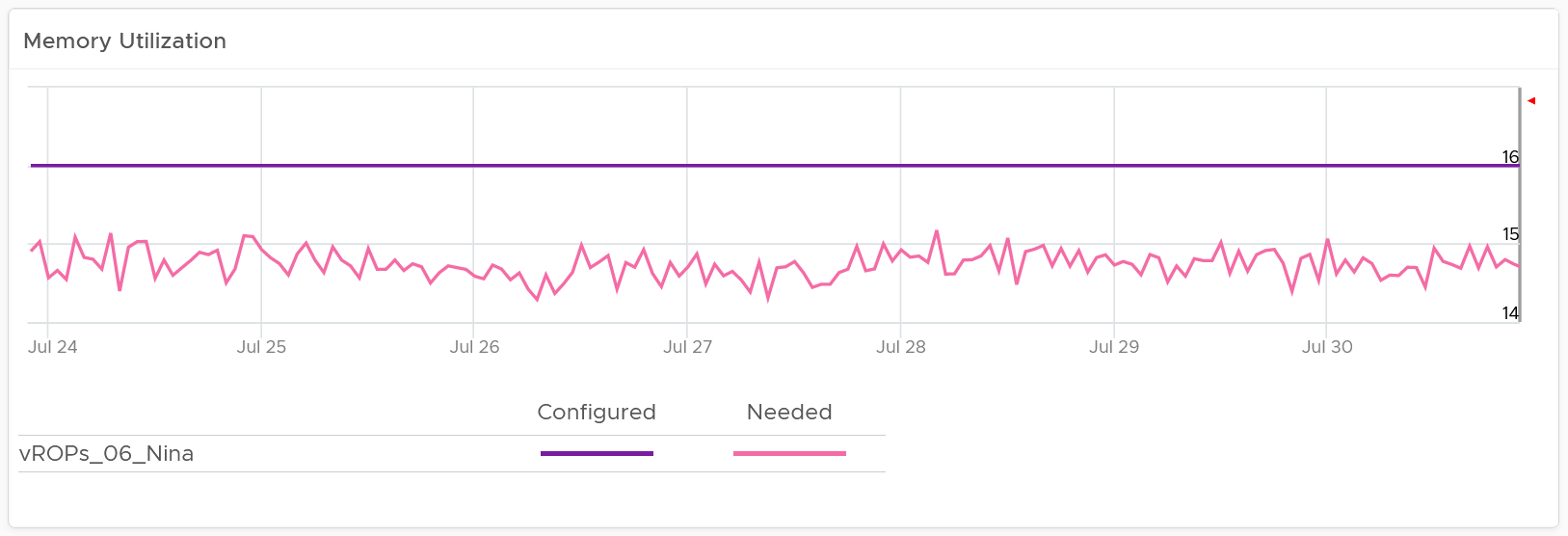
It does not fall back to VM level counter as it’s not a good replacement. See Part 2 Metrics Chapter 3 Memory Metrics.

Rightsizing memory improves performance by reducing memory ballooning and contention. For example, VMs with overprovisioned memory are more likely to experience ballooning

If you want to be conservative, add the free memory counter. If this never touch 0.5 GB, you do not need to add RAM despite its utilization.

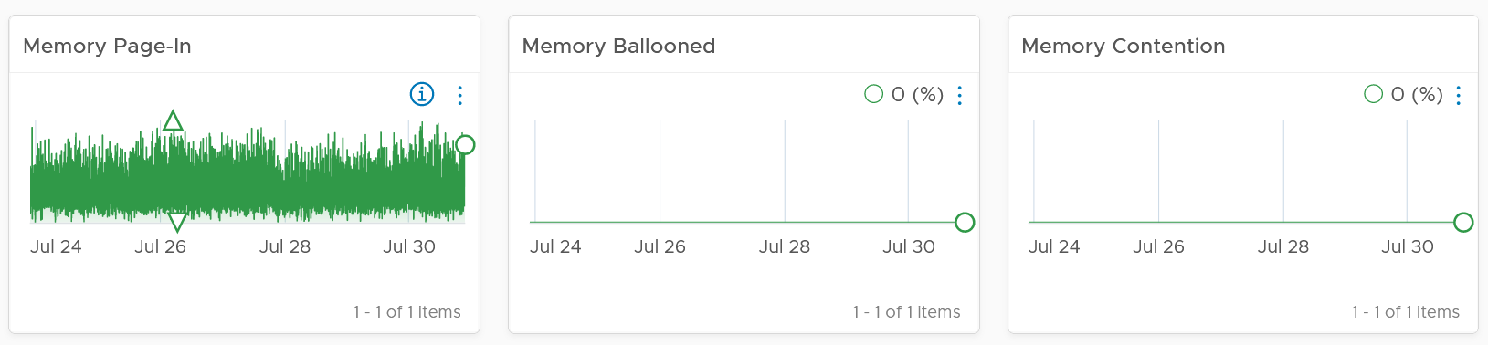
If you have the need, add more metrics such as Page-Out rate.

Relevant configuration for the purpose of right sizing

Points to Note

If your environment is large, change the dashboard filter to a functional filter. Group by the class of services such as gold, silver, and bronze and default the selection to the least critical environment. In this way, you can be more active in reducing the oversized VMs.

For another example, see [Dale Hassinger](https://www.linkedin.com/in/dale-hassinger-5712301b/) at code.vmware.com, where he has more data showing the proof that performance can improve with reduced size.

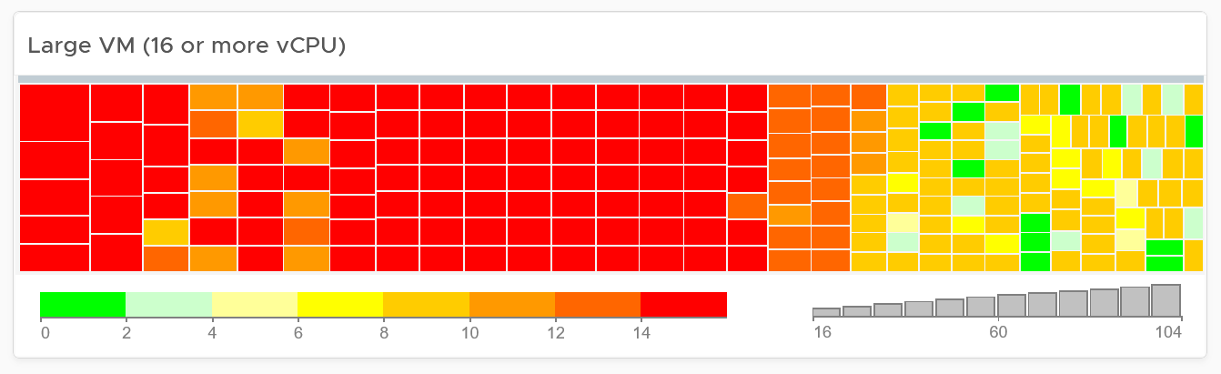
Monster VMs

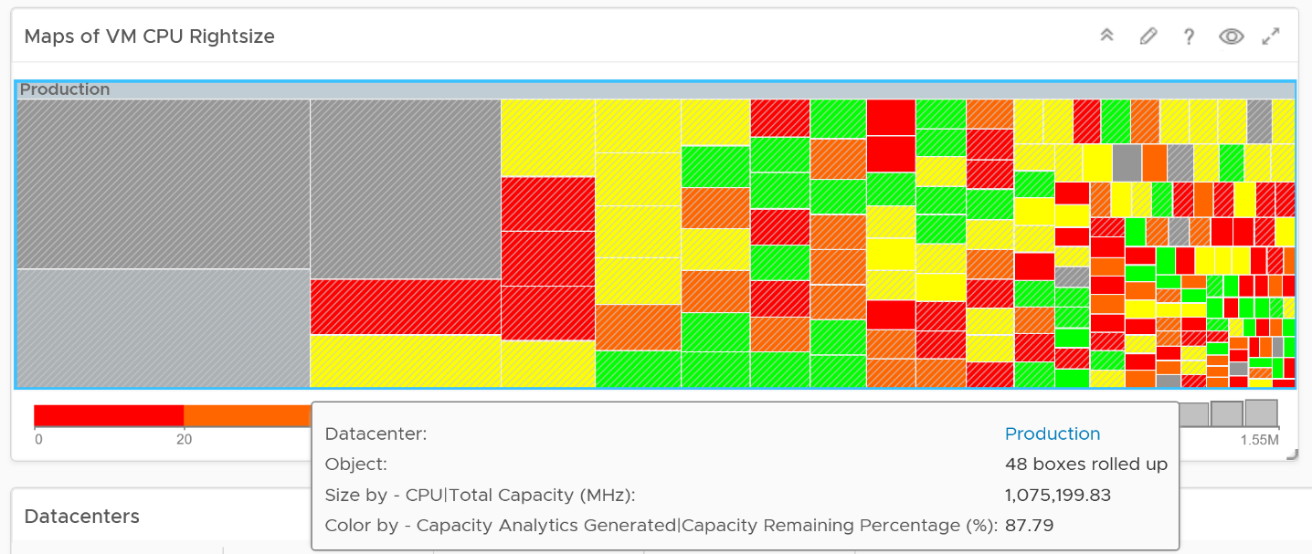
You can enhance the dashboard if you need to convey the overall situation to senior management. You plot every single powered-on VM in the environment, sized by their vCPU. In this way, the monster VMs will be highlighted. A 64 vCPU VM will appear 64x larger than a single vCPU VM. This is good as the focus should be on the large VM, as discussed here.

The heat map colors the VM by its capacity remaining. A VM with high capacity remaining means it has plenty of wastage resources.

What would it look like on an environment with many monster VMs that are oversized? You get something like this. The grey boxes dominate the space of the heat map. One of the boxes consist of 48 VMs with total > 1000 GHz. All of them have 87.79% capacity remaining. Another word, they are oversized.

You may want to do the same for memory.

You can also focus on the large VM by specifying a filter. In the following example, I set to 16 vCPU or more, and the VM has to be powered on at present.

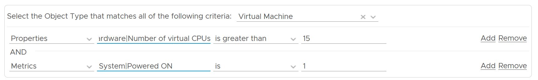
Since we only have the large VM, we can further refine the heat map. The size remains by vCPU size. However, the color changes to the number of oversized vCPU. The more I can reclaim the more red the color shows, and anything above 14 vCPU is red.