Storage

Architecture

To understand storage metrics, be aware that there are 2 dimensions of metrics (speed and space). Both the speed and space dimensions have consumption metrics, but they are completely different.

For speed, the counters are IOPS and throughput, where throughput = IOPS x block size.

For space, the counters are disk space.

Speed

Performance is measured in 2 ways (contention and utilization). Contention can happen at all 3 stages of IO processing: pre-processing: each layer has their own queue or outstanding IO. processing: aborted SCSI commands, dropped frame, etc. post-processing: latency.

Space

Capacity has no impact of slowness in modern, SSD based storage as access to data is no longer relying on spinning platter. 1% disk space full is not slower/faster than 99% full as defragmentation is no longer causing latency. However, it impacts availability. At 100% full, the storage will stop processing IO and your application will crash as a result. Capacity, as in disk space, is measured in bytes. Storage differs to compute as reality overwrites projection. In compute, you use a projected capacity remaining number, which takes into account the past. In storage, if you have 0 bytes left, the number overwrites whatever number shown by capacity engine. You should also focus on reclamation as the amount tends to be substantial.

Storage Layers

Virtualization increases the complexity in both storage capacity and performance. Just like memory, where we have more than 1 level, we have multiple layers of storage and each layer only has control over its own. In addition, each layer may not use the same terminology. For example, the term disk, LUN and device may mean the same thing. A device is typically physical (something you can hold, like an SSD card). LUN is typically virtual, a striping across physical devices in a volume.

The layers present challenge in management, as they create limitation in end-to-end visibility and raise different questions. You lose VM-level visibility in the physical adapter (for example, you cannot tell how many IOPSs on vmhba2 are coming from a particular VM) and physical paths (for example, how many disk commands travelling on that path are coming from a particular VM).

Storage in VMware IaaS is presented as datastore. In some situation, RDM and network file shares are also used by certain VM.

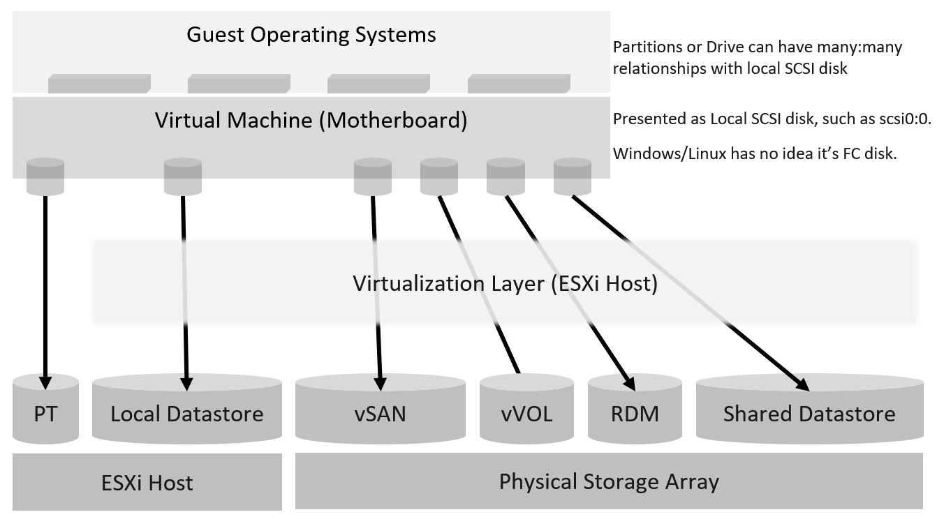
Underlying storage protocol (FC, iSCSI, vSAN, vVOL) is not exposed. Guest OS needs not support the protocol as it’s transparent.

Layer	Description
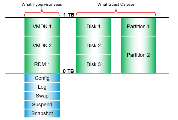
Guest OS	The most upper layer is the Guest OS. It sees virtual disks presented by the VM motherboard. Guest OS typically has multiple partition or drive. Each partition has its own filesystem, serving different purpose such OS drive, paging file drive, and data drive. A large database VM will have even more partitions. Partition may not map 1:1 to the virtual disk. There is no visibility to this mapping. This makes calculating unmapped blocks accurately an impossible task in the case of RDM disk.
	To make it more complex, there is also networked drive. Windows or Linux mounts them over protocol such as SMB. These filesystems are not visible to the hypervisor; hence they are not virtual disk. The disk IO is not visible to the VM as it goes out via vNIC.
VM	See the VM Layer section below
ESXi	See the ESXi Layer section below
Datastore	See the Datastore Layer section below
Storage Subsystem	This can be virtual (e.g. vSAN) or physical (e.g. physical array). If it’s NFS, it can be virtual server or physical. The datastore is normally backed one to one by a LUN, so what we see at the datastore level matches with what we see at the LUN level. Multiple LUNs reside on a single array. Datastores that share the same underlying physical array can experience problem at the same time. The underlying array can experience a hot spot on its own, as it is made of independent magnetic disks or SSD.

VM Layer

The preceding storage layers resulted in 3 different layers of “disks” from the VM downwards. The blue boxes show the 3 layers.

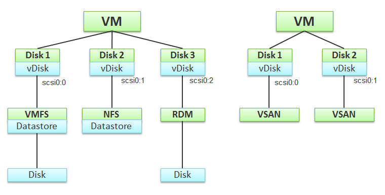
Remember the 3 blue boxes. You will see them, no more no less, in vSphere Client UI. To enable us to focus on the blue boxes, I’ve excluded non virtual disk files such as snapshot and memory swap in the preceding diagram.

The first layer is virtual disk. This exists because the VM does not see the underlying shared storage. It sees as simple local SCSI disks only, as presented by the VM motherboard. This explains why MS-DOS can run on fibre channel, because it’s unaware of the underlying storage architecture.

A virtual disk is identified as scsiM:N, starting with scsi0:0, where M is the adapter bus number.

A virtual disk can sit on top of different underlying storage architecture. I’ve shown 4 in the preceding diagram: NFS, VMFS, vSAN, and RDM. A VM can also be presented with ESXi local physical disk as direct passthrough, although that means the VM cannot run on other ESXi host.

For block datastore (read: VMFS), it can span multiple disks. It is called extend in vSphere. Avoid doing this as it complicates operations. That’s why in the preceding diagram I show a 1:1 relationship.

The discrepancy between VM layer and Guest OS utilization happens because each layer works differently.

• If there is RDM or thick VMDK, VM can’t see the actual used inside Guest OS. It simply sees 100% used, regardless of what Windows or Linux uses.

• If there is unmapped block, Guest OS can’t see this overhead.

We are interested in data both at the VM aggregate level, and at the individual virtual disk level. If you are running a VM with a large data drive (for example, Oracle database), the performance of the data drive is what the VM owner cares about the most. At the VM level, you get the average of all drives; hence, the performance issue could be obscured.

Metric Mapping

While there is a 1:1 mapping between Guest OS and its underlying VM, not all metrics map. The following table explains it:

Type	Guest OS Metrics	VM Metrics
Contention	OS Queue	None, as VM is not an OS. Because it is a motherboard, the driver is specific to the Guest OS.
	Driver Queue
	Latency	Latency. They should be similar, especially when plotted over time.
Utilization	IOPS	They should match with the metrics at VM level, especially when plotted over time. If not, there is something wrong.
	Throughput

Performance

Latency can happen when IOPS and throughput are not high, because there are multiple stacks involved and each stack has their own queue. It begins with a process, such as a database, issuing IO request. This gets processed by Windows or Linux storage subsystem, and then send to the VM storage driver.

Ensure that you do not have packet loss for your IP Storage, dropped FC frames for FC protocol, or SCSI commands aborted for your block storage. They are a sign of contention as the datastore (VMFS or NFS) is shared. The metrics Bus Resets and Commands Aborted should be 0 all the time. As a result, it should be fine to track them at higher level objects. Create a super metric that tracks the maximum or summation of both, and you should expect a flat line.

Once you have ensured that you do not have packet loss on IP Storage or aborted commands on block storage, use the latency counter and outstanding IO for monitoring. For troubleshooting, you will need to check both read latency and write latency, as they tend to have different patterns and value. It’s common to only have read or write issue, and not both.

Total Latency is not (Read Latency + Write Latency) / 2. It is not a simple summation. In a given second, a VM issues many IOPS. For example, the VM issues 100 reads and 10 writes in a second. Each of these 110 commands will have their own latency. The “total” latency is the average of these 110 commands. In this example, the total latency will be more influenced by the read latency, as the workload is read dominated.

If you are using IP storage, take note that Read and Write do not map 1:1 to Transmit (Tx) and Receive (Rx) in Networking metrics. Read and Write are both mapped to Transmit counter as the ESXi host is issuing commands, hence transmitting the packets.

Capacity

A VM can consume storage via:

• Virtual disk.\

  Each virtual disk has label, type (RDM or VMDK), provisioning type (thin, lazy zero, eager zero). If it’s RDM, need to know additional properties such as RDM type (physical or virtual).

• Compute virtualization.\

  Snapshots, Swapped, Logs. Guest OS can’t see them.This can be overhead and non-overhead. This is not visible to the Guest OS. They are shown in blue in the following diagram.

• Storage virtualization.\

  This includes vSAN protection, deduplication and decompression. We need this number to reported separately as it’s not applicable in non vSAN.

There are more file types than shown above. However, from monitoring and troubleshooting viewpoint, the above is sufficient.

ESXi Layer

Storage at ESXi is more complex than storage at VM level. Reason is ESXi virtualizes the different physical storage subsystem, and VM simply consumes all of them as local SCSI drive. The kernel does the IO on behalf of all the VMs. It also has its own kernel modules, such as vSAN.

Typically, multiple VMs run on the same ESXi, and multiple ESXi hosts mount a shared datastore. This creates what is popularly termed “IO Blender” effect. Sequential operations from each VM and kernel modules become random when combined together. The opposite is when the kernel rearranges these independent IOs and try to sequence them, so on average the latency is lower.

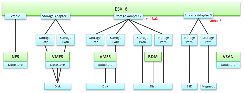
The green boxes are what you are likely to be familiar with. You have your ESXi host, and it can have NFS Datastore, VMFS Datastore, vSAN Datastore, vVOL datastore or RDM objects. vSAN & vVOL present themselves as a VMFS datastore, but the underlying architecture is different. The blue boxes represent the metric groups you see in vCenter performance charts.

Just like compute virtualization, there is no more association to VM for metrics at physical layers.

In the central storage architecture, NFS and VMFS datastores differ drastically in terms of metrics, as NFS is file-based while VMFS is block-based.

• For NFS, it uses the vmnic, and so the adapter type (FC, FCoE, or iSCSI) is not applicable. Multipathing is handled by the network, so you don't see it in the storage layer.

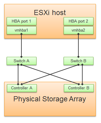
• For VMFS or RDM, you have more detailed visibility of the storage. To start off, each ESXi adapter is visible and you can check the metrics for each of them. In terms of relationship, one adapter can have many devices (disk or CDROM). One device is typically accessed via two storage adapters (for availability and load balancing), and it is also accessed via two paths per adapter, with the paths diverging at the storage switch. A single path, which will come from a specific adapter, can naturally connect one adapter to one device. The following diagram shows the four paths:

The counter at ESXi level contains data from all VMs and the kernel overhead. There is no breakdown. For example, the counter at vmnic, storage adapter and storage path are all aggregate metrics. It’s not broken down by VM. The same with vSAN objects (cache tier, capacity disk, disk group). None of them shows details per VM.

Can you figure out why there is no path to the VSAN Datastore?

We’ll do a comparison, and hopefully you will realize how different distributed storage and central storage is from performance monitoring point of view. What look like a simple change has turned the observability upside down.

Storage Adapter

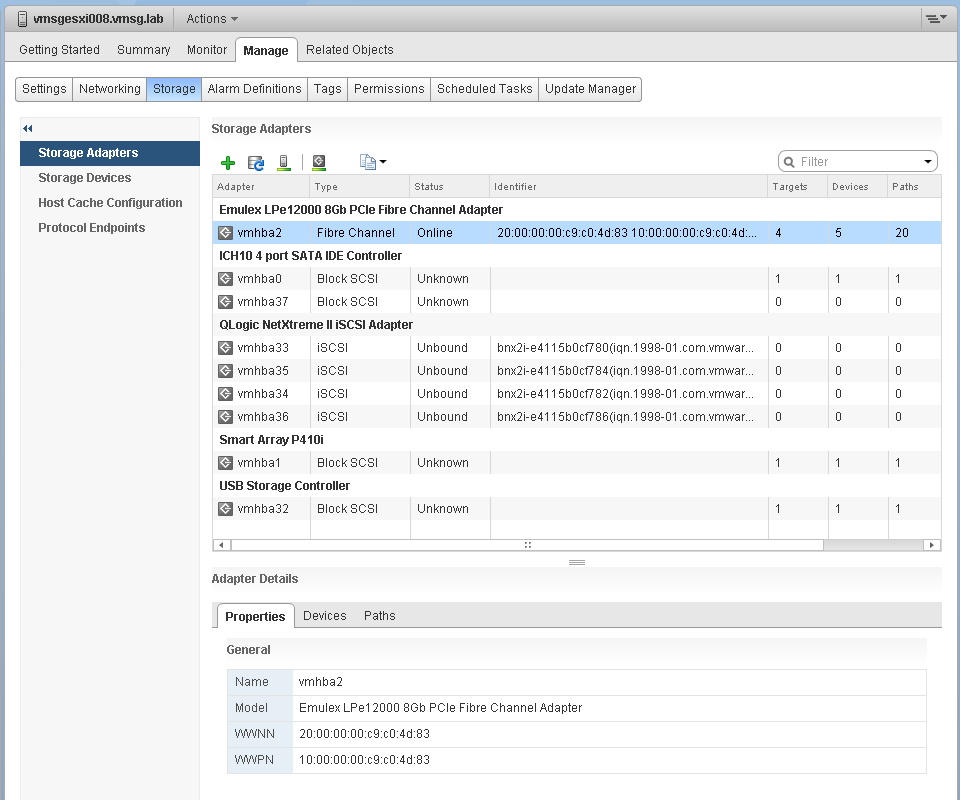
The screenshot shows an ESXi host with the list of its adapters. We have selected vmhba2 adapter, which is an FC HBA. Notice that it is connected to 5 devices. Each device has 4 paths, giving 20 paths in total.

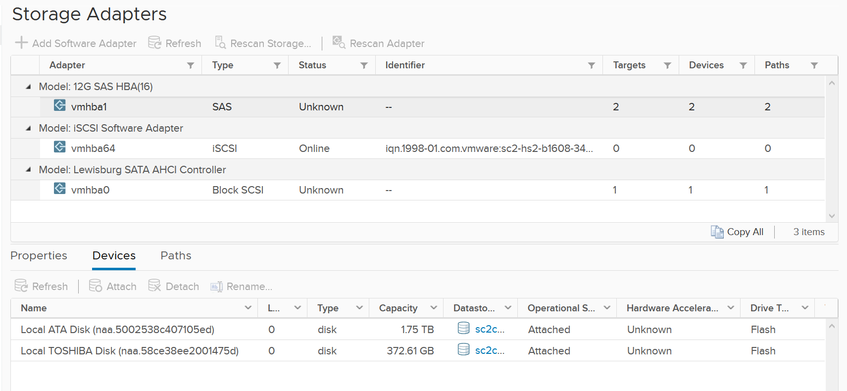
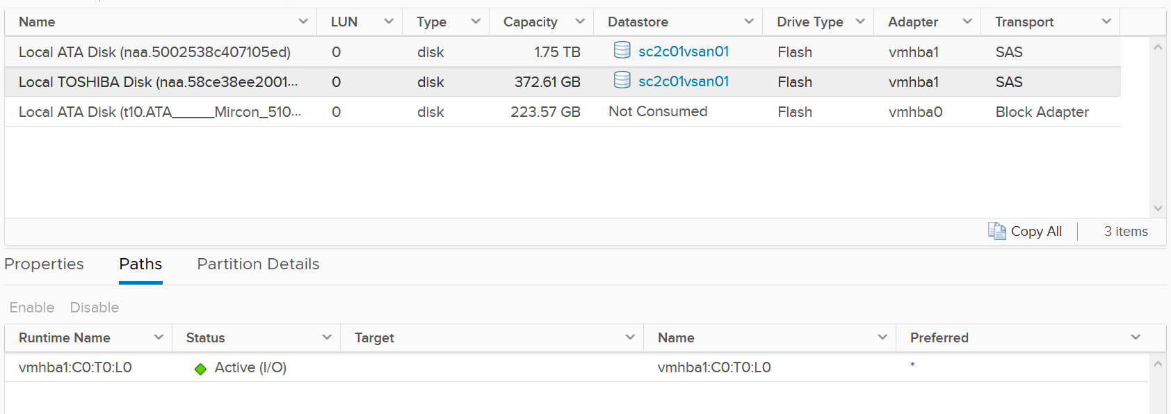
What do you think it will look like on vSAN? The following screenshot shows the storage adapter vmhba1 being used to connect to two vSAN devices. Both devices have names begin with “Local”. The storage adapter has 2 targets, 2 devices and 2 paths. If you are guessing it is 1:1 mapping among targets, devices and paths, you are right.

We know vSAN is not part of Storage Fabric, so there is no need for Identifier, which is made of WWNN and WWPN.

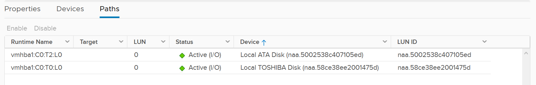
Let’s expand the Paths tab. We can see the LUN ID here. This is important. The fact that the hypervisor can see the device is important. That means the kernel can report if there is an issue, be it performance or availability. This is different if the disk is directly passed through to the VM. The hypervisor loses visibility.

Storage Path

Continuing our comparison, the last one is Storage Path. In a fibre channel device, you will be presented with the information shown in the next screenshot, including whether a path is active or not.

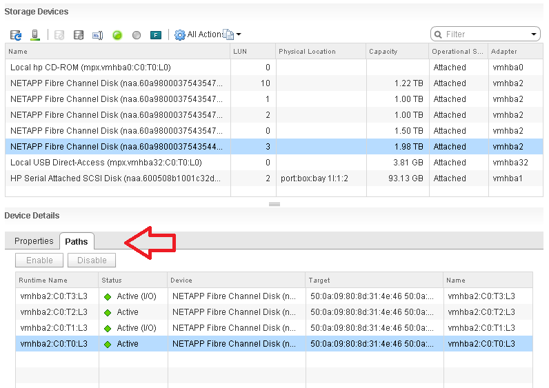
Note that not all paths carry I/O; it depends on your configuration and multipathing software. Because each LUN typically has four paths, path management can be complicated if you have many LUNs.

What does Path look like in vSAN? As shared earlier, there is only 1 path.

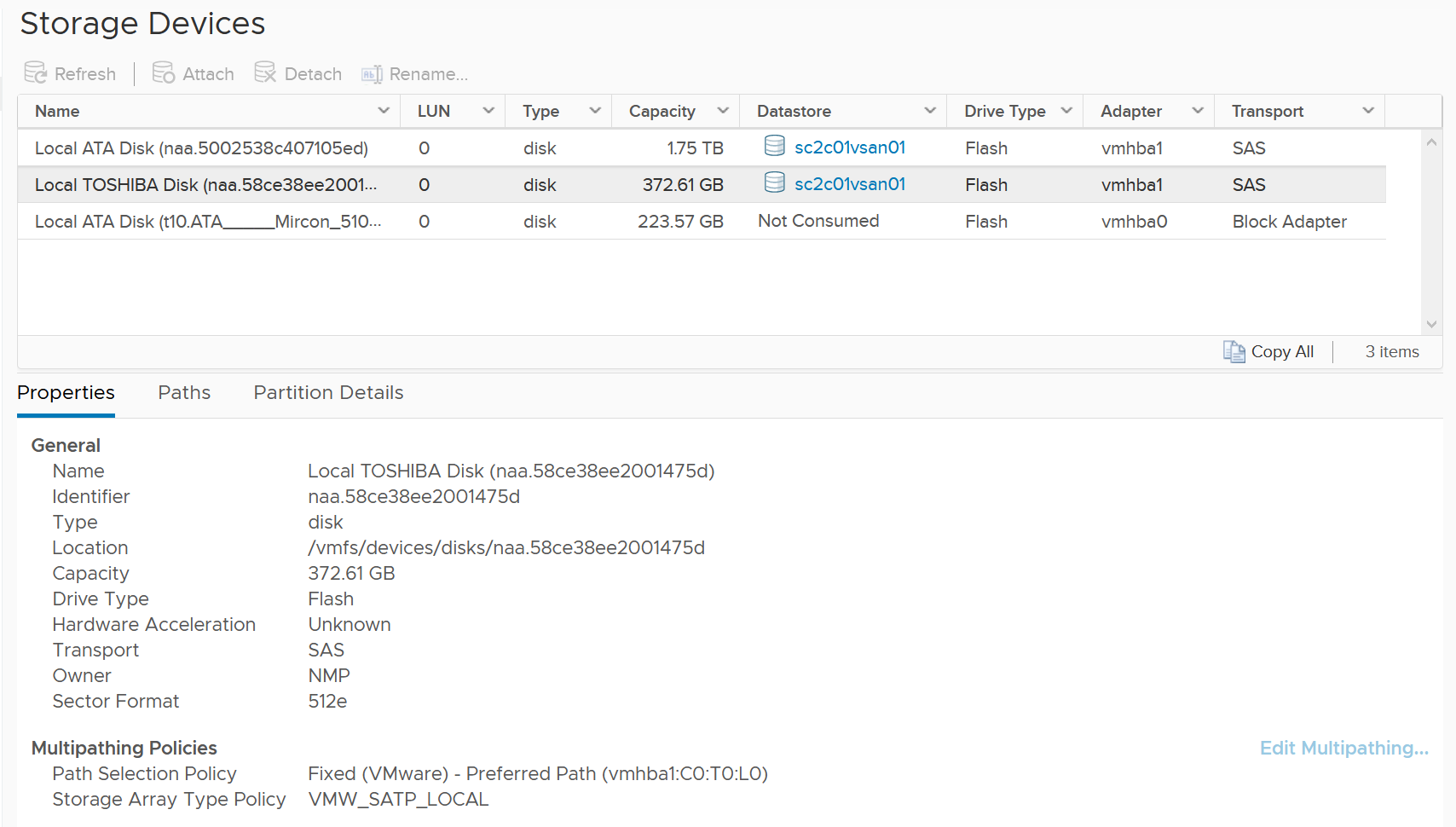
Storage Devices

The term drive, disk, device, storage can be confusing as they are often used interchangeably in the industry. vSphere Client uses the terms device and disk interchangeably. In vSphere, this means a physical disk or physical LUN partition presented to ESXi host.

The following shows that the ESXi host has 3 storage devices, all are flash drive and the type = disk. The first two are used in vSAN datastore and are accessed via the adapter vmhba1.

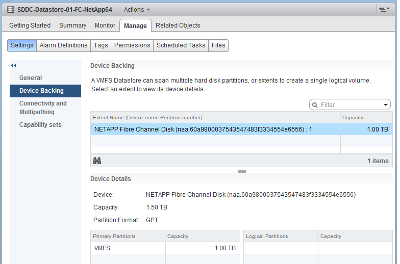
A storage path takes data from ESXi to the LUN (the term used by vSphere is Devices), not to the datastore. So if the datastore has multiple extents, there are four paths per extent. This is one reason why you should not use more than one extent, as each extent adds 4 paths. If you are not familiar with VMFS Extent, Cormac Hogan explains it here.

For VMFS (non vSAN), you can see the same metrics at both the Datastore level and the Disk level. Their value will be identical if you follow the recommended configuration to create a 1:1 relationship between a datastore and a LUN. This means you present an entire LUN to a datastore (use all of its capacity). The following shows a VMFS datastore with a NetApp LUN backing it.

In vSAN, there is no connectivity and Multipathing menu. There is also no Capability Sets menu. vSAN datastore is not mapped to a LUN. It is supported by disk groups.

Datastore Layer

What you can see at this level, and hence how you monitor, depends on the storage architecture.

The underlying storage protocol can be files (NFS) or blocks (VMFS). vSAN uses VMFS as its consumption layer as the underlying layer is unique to vSAN, and hence vSAN requires its own monitoring technique. Because vSAN presents itself as a VMFS datastore you need to know that certain metrics will behave differently when datastore type is vSAN.

For VMFS datastore, the VM IO commands are passed down as is to the Pluggable Storage Architecture (PSA) layer. There is one queue (schedQ) made for each vmdk on each VM. The metrics at this layer is are collected at that layer.

For NFS datastore, as it is network file share (as opposed to block), you have no visibility to the underlying storage. The type of metrics will also be more limited, and network metric becomes more critical.

Relationship

A datastore has relationship to 3 other objects:

• VM

• ESXi

• Cluster

A datastore typically has 1:M relationship to VM. It is also typically shared by multiple ESXi. If you design such that a VM spans multiple datastores, and a datastores spans multiple clusters, you create a trade-off in terms of observability.

The value of datastore metric excludes VMDK that is not on the datastore. It includes every files in the datastore, including orphaned files outside the VM folder. Logically, it also excludes RDM.

I created a simple diagram below, with just 4 VMs on 2 ESXi and 2 datastores. What complications do you see?

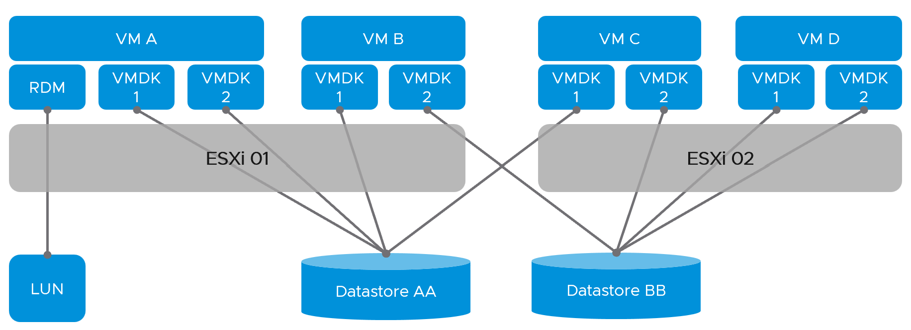
Performance and capacity become complex due to many to many relationships. The metrics at ESXi level and cluster will not match the metrics at datastore level. How do you then aggregate the cluster storage capacity when its datastores are shared with other clusters?

You’re right. You can’t.

In summary, while there are use cases where you should separate the VMDK into multiple datastores, take note of the observability compromise.

Backing Device

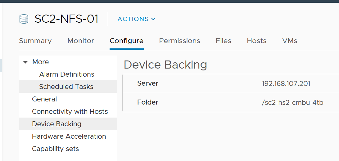
Since datastore is a filesystem, it’s necessary to monitor the backing device. This can be NFS or LUN. For NFS, it looks something like this:

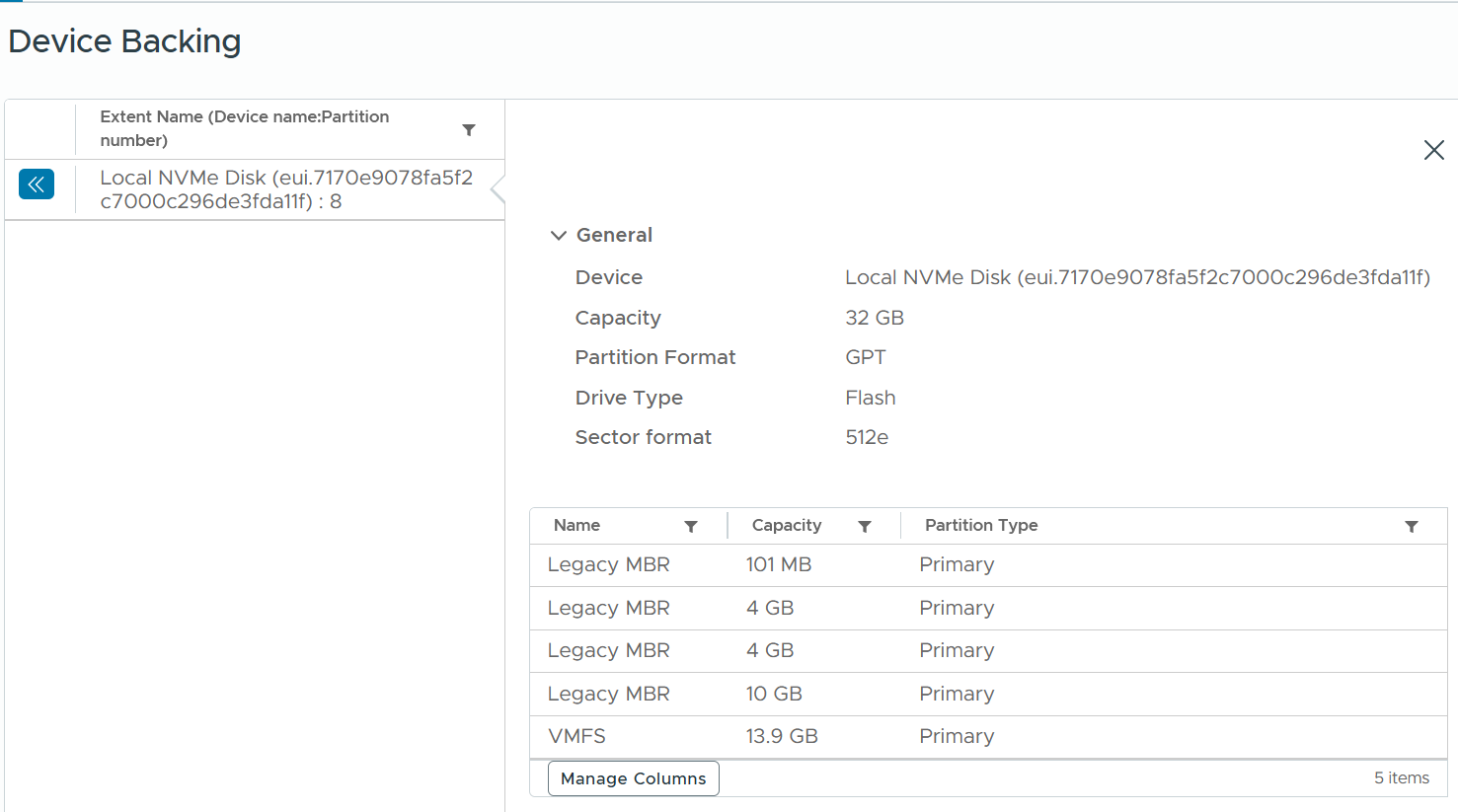
For a local disk, it looks something like this:

Since the underlying device is outside the realm of vSphere, you need to login to the storage provider and build the relationship. Compare the metrics by deriving a ratio. Investigate if this ratio shows unexpected value.

Take for example, a datastore on a FC LUN. If you divide the IOPS at the LUN level with the IOPS at the datastore, what value do you expect?

Assuming they are mapped 1:1, then the ratio should be 1.

If the value is > 1, that means there are IO operations performed by the array. This could be array level replication or snapshot.

What about NFS datastores? The troubleshooting is different as you now need to at files as opposed to block. In both cases, you need to monitor the filer or array directly.

VM

We covered earlier that storage differs to compute as it covers both dimensions (speed and space). As a result, we cannot simply use the contention and consumption as grouping. Instead we would group by performance and capacity. This is also good as operationally you manage performance and capacity differently.

Overview

Recall the 3 layers of storage from VM downward. As stated, the 3 blue boxes appear in the vSphere Client UI as virtual disk, datastore and disk.

Among the 3, which one is the most important?

You’re right, virtual disk.

It is the closest to the VM and it is the most detail in terms of observability.

Virtual Disk

Use the virtual disk metrics to see VMFS vmdk files, NFS vmdk files, and RDMs.

However, you don’t get data for anything other than virtual disk. For example, if the VM has snapshot, the metric does not include the snapshot data.

A VM typically has multiple virtual disks, typically 1 Guest OS partition maps to 1 virtual disk. The following VM has 3 virtual disks.

As you can see in the preceding screenshot of vSphere Client UI, there is no aggregate number at VM level. You need to add them manually in vCenter. In VCF Operations, you use the “aggregate of all instances” metric to see the rest.

The following properties is available in VCF Operations for each virtual disk:

Property Name	Values
Virtual Device Node	Virtual disks SCSI bus location. Virtual disks are enumerated starting with the first controller and moving along the bus.
Compatibility Mode	Physical Virtual Virtual mode specifies full virtualization of the mapped device. Physical mode specifies minimal SCSI virtualization of the mapped device.
Disk Mode	Dependent Independent – Persistent Independent – Nonpersistent
SCSI Bus Sharing	None Physical Virtual
SCSI Controller Type	BusLogic Parallel LSI Logic Parallel LSI Logic SAS VMware Paravirtual
Encryption Status
Is RDM	true false False means the virtual disk is a VDMK not RDM.
Virtual Disk Sharing	Unspecified No Sharing Multi-Writer

The property “Number of VDMK” excludes RDM, as the name implies. The metric “Number of RDMs” only includes RDM attached to the VM.

Pro Tip: sum the property “Number of RDMs” from all the VMs in a single physical storage array. Compare the result with the number of LUNs in the array that are carved out for RDM purpose. If there are more LUNs than this number, you have unused RDM.

You need to do the above per physical array, so you know which array needs attention.

Disk

This should be called Physical Disk or Device, as a simple terminology “disk” sounds like a superset of virtual disk.

Disk means device, so we’re measuring at LUN level or RDM level. It’s great to know that we can associate the metrics back to the VM. Notice we can’t associate it to specific virtual disk as they are different layers.

Use the disk metrics to see VMFS and RDM, but not NFS. The data at this level should be the same as at Datastore level because your blocks should be aligned; you should have a 1:1 mapping between Datastore and LUN, without extents. It also has the Highest Latency counter, which is useful in tracking peak latency

The metric is at the disk level. So I’m not 100% sure if the value is per VM or per disk (which typically has many VM).

Raw Device Mapping

RDM appears clearly as LUN in the VM Edit Settings dialog box:

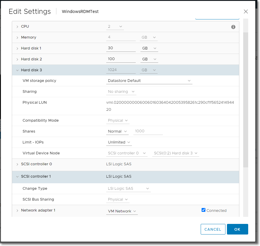
But what does it appear when you browse the VM folder in the parent datastore?

RDM appears like a regular VMDK file. There is no way to distinguish it in the folder.

Datastore

Use the datastore metrics to see VMFS and NFS, but not RDM. Because snapshots happen at Datastore level, the counter will include it. Datastore figures will be higher if your VM has a snapshot. You don’t have to add the data from each virtual disk together as the data presented is already at the VM level. It also has the Highest Latency counter, which is useful in tracking peak latency.

Just like LUN level, we lose the breakdown at virtual disk. The metric is only available at VM level.

Mapping

If all the virtual disks of a VM are residing in the same datastore, and that datastore is backed by 1 LUN, then all the 3 layers will have fairly similar metrics. The following VM has 2 virtual disks (not shown). Notice all 3 metrics are identical over time.

The difference comes from files outside the virtual disks, such as snapshot, log files, and memory swap.

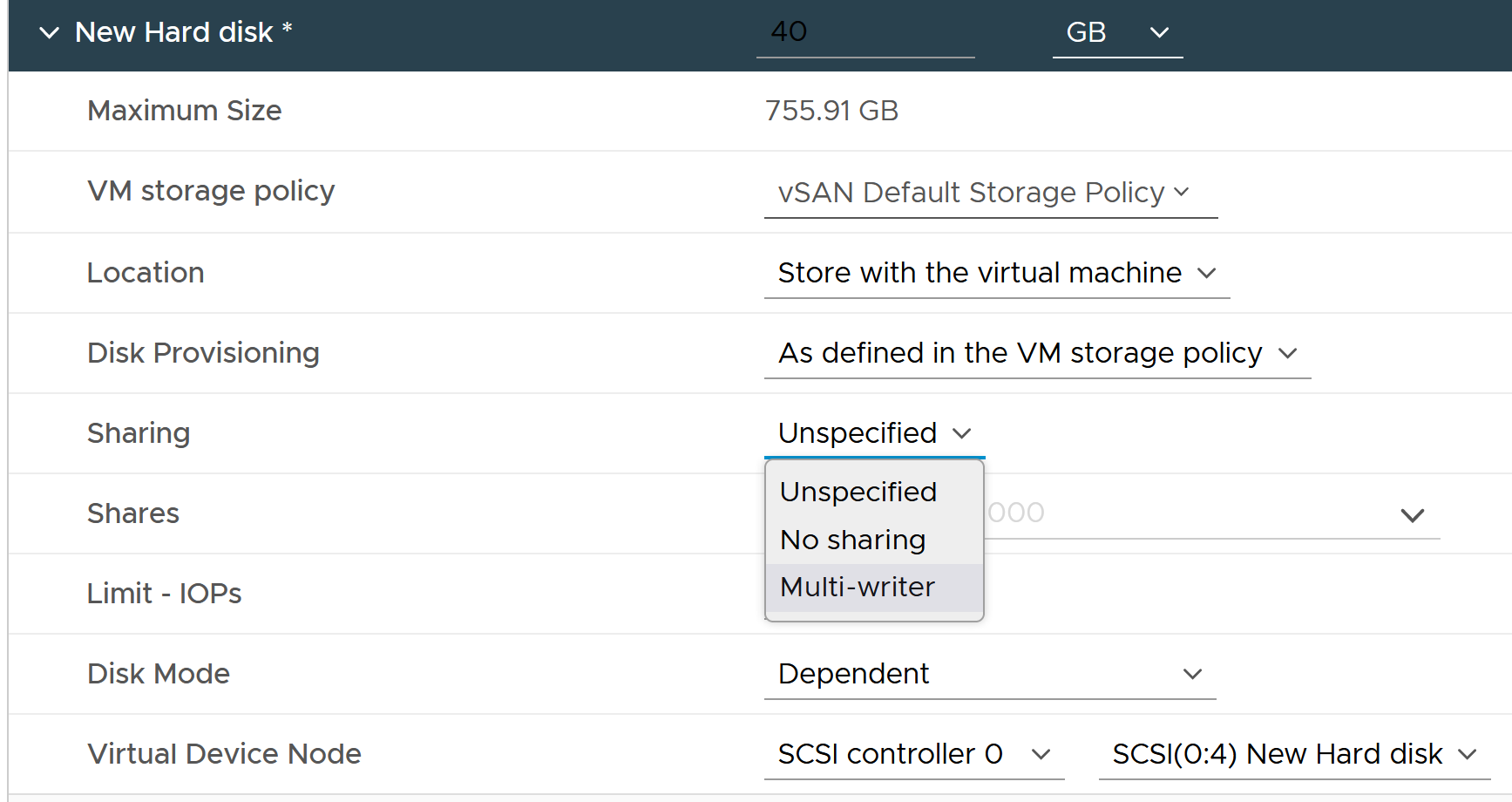
Multi-Writer Disk

In application such as database, multiple VMs need to share the same disk.

Shared disk can be either shared RDM or VMDK. The following screenshot shows the option when creating a multi-writer VMDK in vCenter Client.

When multiple VMs are sharing the same virtual disk or RDM, it creates additional challenge in capacity, cost and performance management. In the following example, notice the metric become flat 0. See the red arrow.

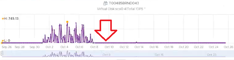
The above is obviously wrong as IOPS are typically not flat 0.

What happens here is typical Active/Passive pair of VM. The application fail over to the second VM, so the first VM becomes passive. vCenter API returns 0 instead of blank, hence you see 0 in VCF Operations.

You can see from the following screenshot that the second VM took over at the time the first VM failover. Notice it started showing IOPS metrics on the same time.

Do you notice something inconsistent?

The first VM returns 0 after failover. The second VM returns blank (no data) before taking over.

Metrics

Name	Description
Disk Space | Active Not Shared (GB)	The total amount of disk space from all the VMDK and RDM that are exclusively owned by this VM. Active only cover the virtual disks. Snapshot is considered as non-active files hence it’s not counted. Formula: Disk Space|Not Shared (GB) - Disk Space|Snapshot Space (GB)

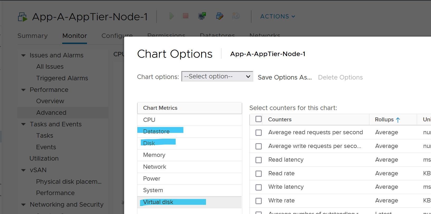
Performance Metrics

Just like CPU and memory, we would cover contention type of metric first, then the consumption type of metrics.

Contention Metrics

Contention could happen due to the VM itself (e.g. IOPS Limit has been placed) or the underlying infrastructure.

We will cover them from virtual disk first, then datastore and disk.

Virtual Disk

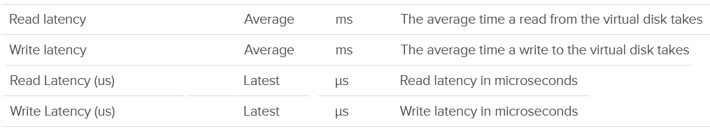
The main metrics for tracking performance is latency. They are provided in both ms and microsecond.

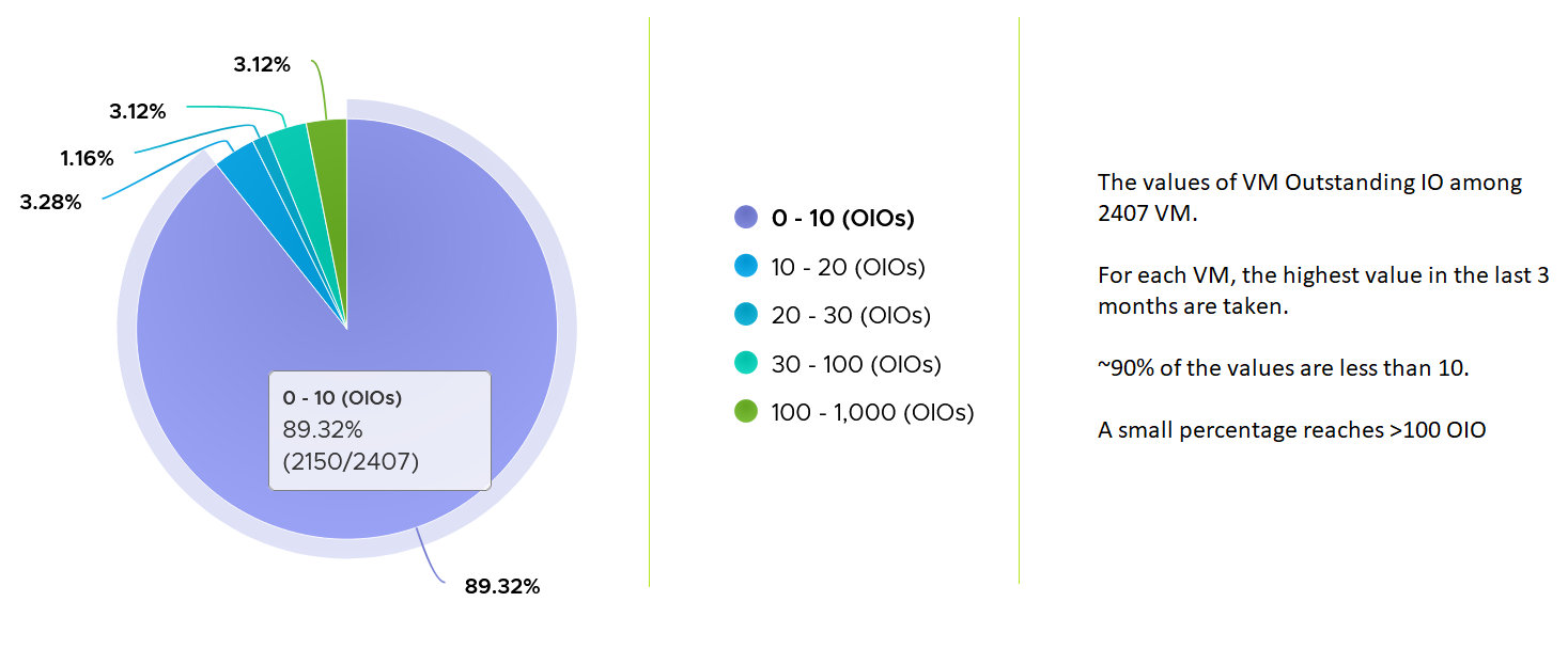
A related counter to latency is Outstanding IO.

This is the number of I/Os that have been issued, but not yet completed. They are waiting in the queue, indicating a bottleneck

The relationship is

Average Latency = Average Outstanding IO / Average IOPS

Outstanding IO should be seen in conjunction with latency. It can be acceptable to have high number of IO in the queue, so long the actual latency is low.

Since your goal is maximum IOPS and minimum latency, the metric is less useful as its value is impacted by IOPS. See this KB article for VSAN specific recommendation on the expected value.

What should be the threshold value?

That depends on your storage, because the range varies widely. Use the profiling technique to establish the threshold that is suitable for your environment.

In the following analysis, we take more than 63 million data points (2400 VM x 3 months worth of data). Using data like this, discuss with the storage vendor if that’s in line with what they sold you.

Disk

As the physical disk layer, there are 2 error metrics. I always find their values to be 0 all the time, so if you’ve seen a non-zero value let me know.

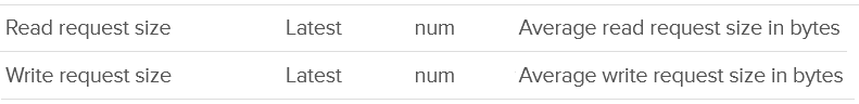
For latency, there is no breakdown. It’s also the highest among all disks. Take note the roll-up is latest, so it’s the single value at the end of the collection period.

Datastore

At the datastore layer, the only metric provided for contention is latency. There is no outstanding IO.

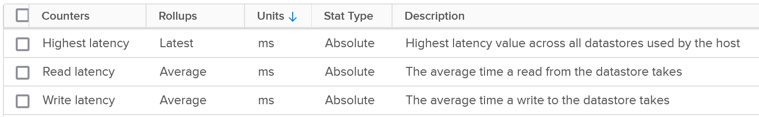
The highest latency is useful for VMs with multiple datastores. But take note the roll-up is Latest, not average.

For the read and write latency, the value in VCF Operations is a raw mapping to these values datastore.totalReadLatency.average and datastore.totalWriteLatency.average

Consumption metrics

A typical suspect for high latency is high utilization, so let’s check what IOPS and throughput metrics are available.

Virtual Disk

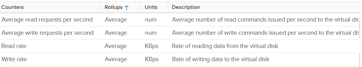
As you can expect, you’re given both IOPS and throughput metrics at virtual disk level.

VM Disk IOPS and throughput vary widely among workload. For a single workload or VM, it also depends on whether you measure during its busy time or quiet time.

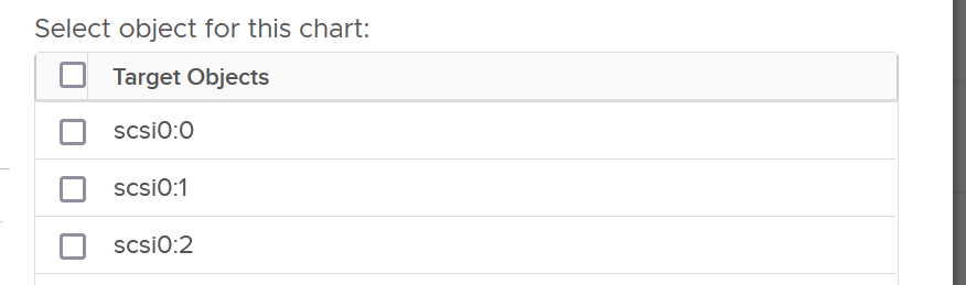
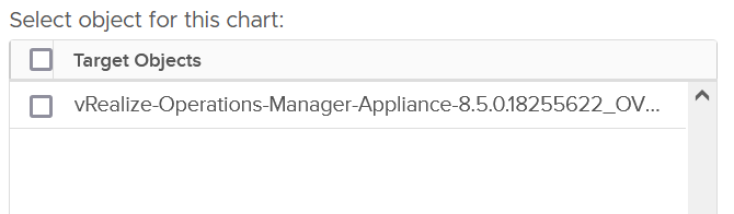
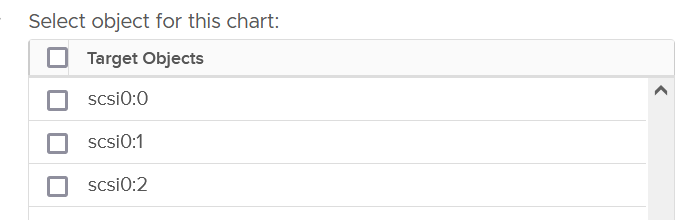
Take note that vSphere Client does not provide summary at VM level. Notice the target objects are individual scsiM:N, and there is no aggregation at VM level as the option in Target Objects column below.

In the following example, I plotted from a 3500 production VMs. They are sorted by the largest IOPS on any given 5 minute. What’s your take?

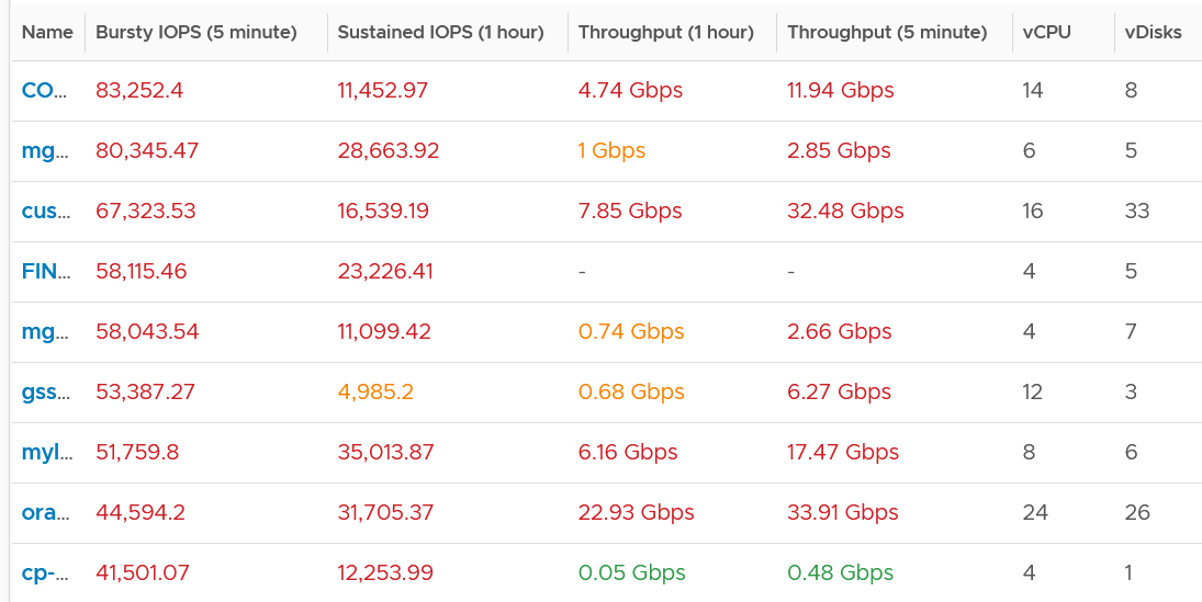
I think those numbers are high. At 1000 IOPS averaged over 5 minutes, that means 300,000 total IO commands that need to be processed. So 10K IOPS translates into 3 millions commands, which must be completed within 300 seconds.

A high IOPS can also impact the pipe bandwidth, as it’s shared by many VMs and the kernel. If a single VM chews up 1 Gb/s, you just need a handful of them to saturate 10 Gb ethernet link.

There is another problem, which is sustained load. The longer the time, the higher the chance that other VMs are affected.

In the following example, it’s a burst IOPS. Regardless, discuss with the application team if it is higher than expected. What’s normal from one application may not be for another.

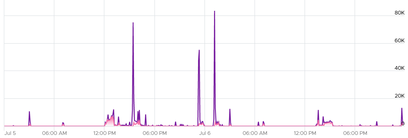
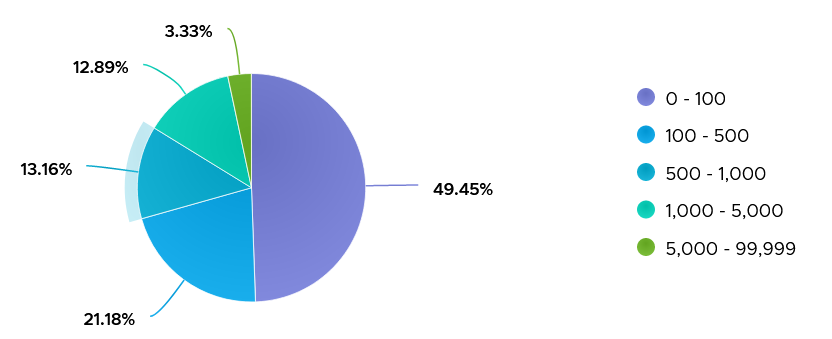
While there is no such thing as normal distribution or range, you can analyse your environment so you get a sense. I plotted all the 3500 VMs and almost 85% did not exceed 1000 IOPS in the last 1 week. The ones hitting >5K IOPS only form around 3%.

If the IOPS is low, but the throughput is high, then the block size is large. Compare this with your expected block size, as they should not deviate greatly from plan. You do have a plan, don’t you 😉

You can set the limit for individual virtual disk of VM.

A few rows below, and you will see the following.

The default setting is no limit, which is what I recommend.

Note that the limit on a virtual disk, not the whole VM. That means you cannot set limit on non virtual disk such as snapshot and memory swap. This makes sense as they are part of IaaS.

Take note that since the limit is applied at VM level, the metrics that will show high latency is at Guest OS levels. The VM metric will not show high latency, as the IO that were allowed to pass was not affected by this limit. This is no different to any problem at Guest OS layer. For example, if LSI Logic or PVSCSI driver is causing problem, the VM will not report anything as it’s below the Guest OS driver.

VCF Operations have the following related data at each virtual disk

• IOPS Limit property.

• IOPS per GB metric.

Disk

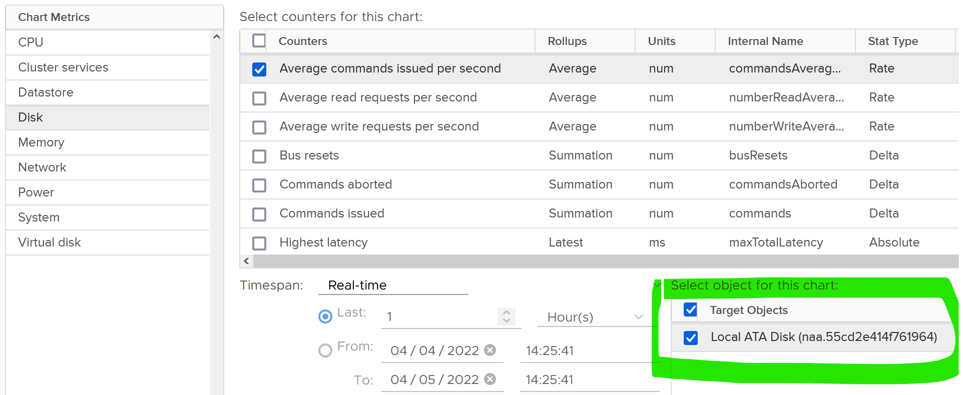
There are 2 sets of metrics for IOPS. Both are basically the same. One if the total number of IO in the collection period, while the other one is average of 1 second.

There are the usual metrics for throughput.

It will be great to have block size, especially the maximum one during the collection period.

Datastore

For utilization, both IOPS and throughput are provided.

For the IOPS, the value in VCF Operations is a raw mapping to these values datastore.numberReadAveraged.average and datastore.numberWriteAveraged.average in vCenter.

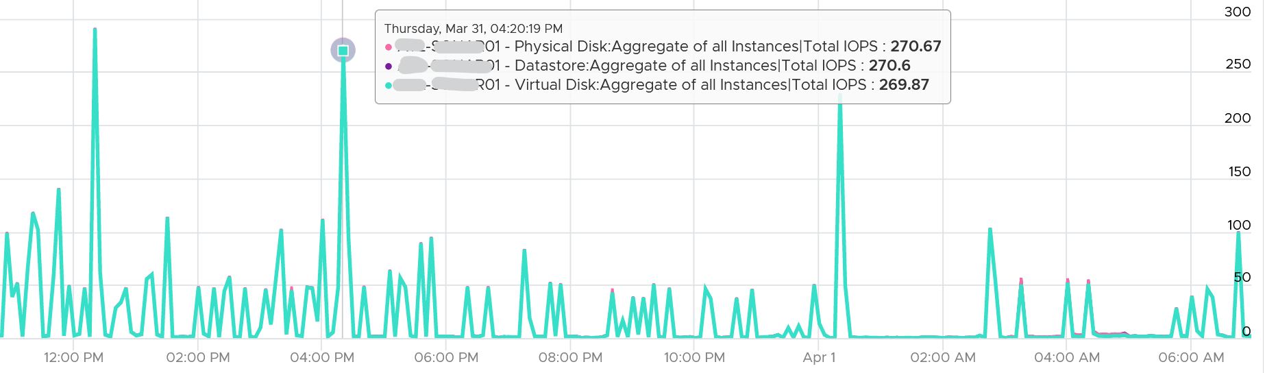
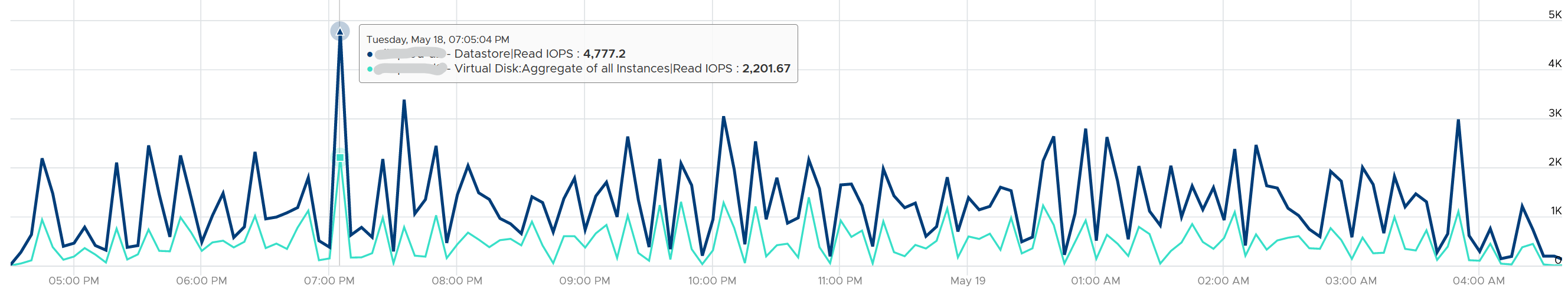
Review the following screenshot. Notice something strange among the 3 metrics?

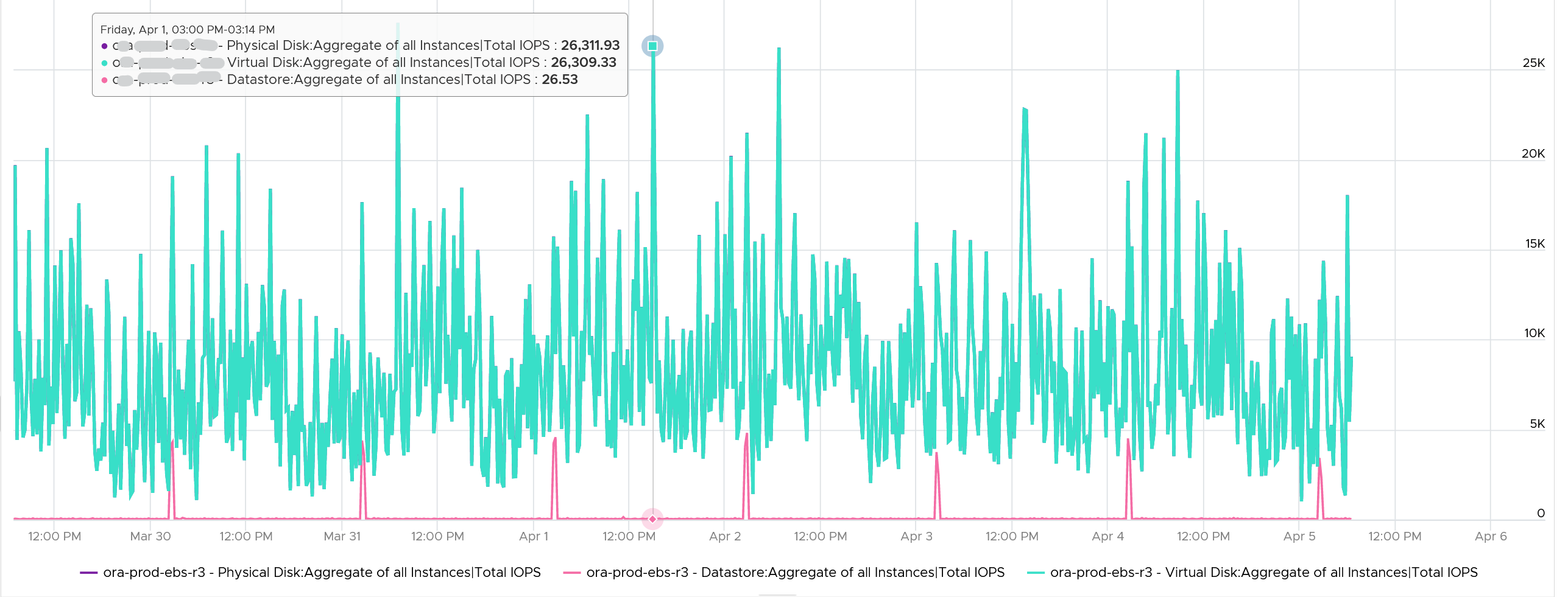
Yes, the total IOPS at datastore level is much lower than the IOPS at physical disk and virtual disk levels. The IOPS at physical disk and virtual disk are identical over the last 7 days. They are quite active.

The IOPS at datastore level is much lower, and only spike once a day. This VM is an Oracle EBS VM with 26 virtual disks. Majority of its disks are RDM, hence the IOPS hitting the datastore is much less.

Snapshot requires additional read operations, as the reads have to be performed on all the snapshots. The impact on write is less. I’m not sure why it goes up so high, but logically it should be because many files are involved. Based on the manual, a snapshot operation creates .vmdk, -delta.vmdk, .vmsd, and .vmsn files. Read more here.

For Write, ESXi just need to write into the newest file.

The pattern is actually identical. I take one of the VM and show it over 7 days. Notice how similar the 2 trend charts in terms of pattern.

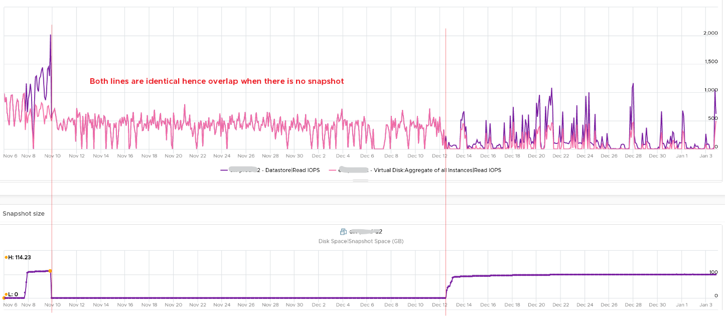
You can validate if snapshot causes the problem by comparing before and after snapshot. That’s exactly what I did below. Notice initially there was no snapshot. There was a snapshot briefly and you could see the effect immediately. When the snapshot was removed, the 2 lines overlaps 100% hence you only see 1 line. When we took the snapshot again, the read IOPS at datastore level is consistently higher.

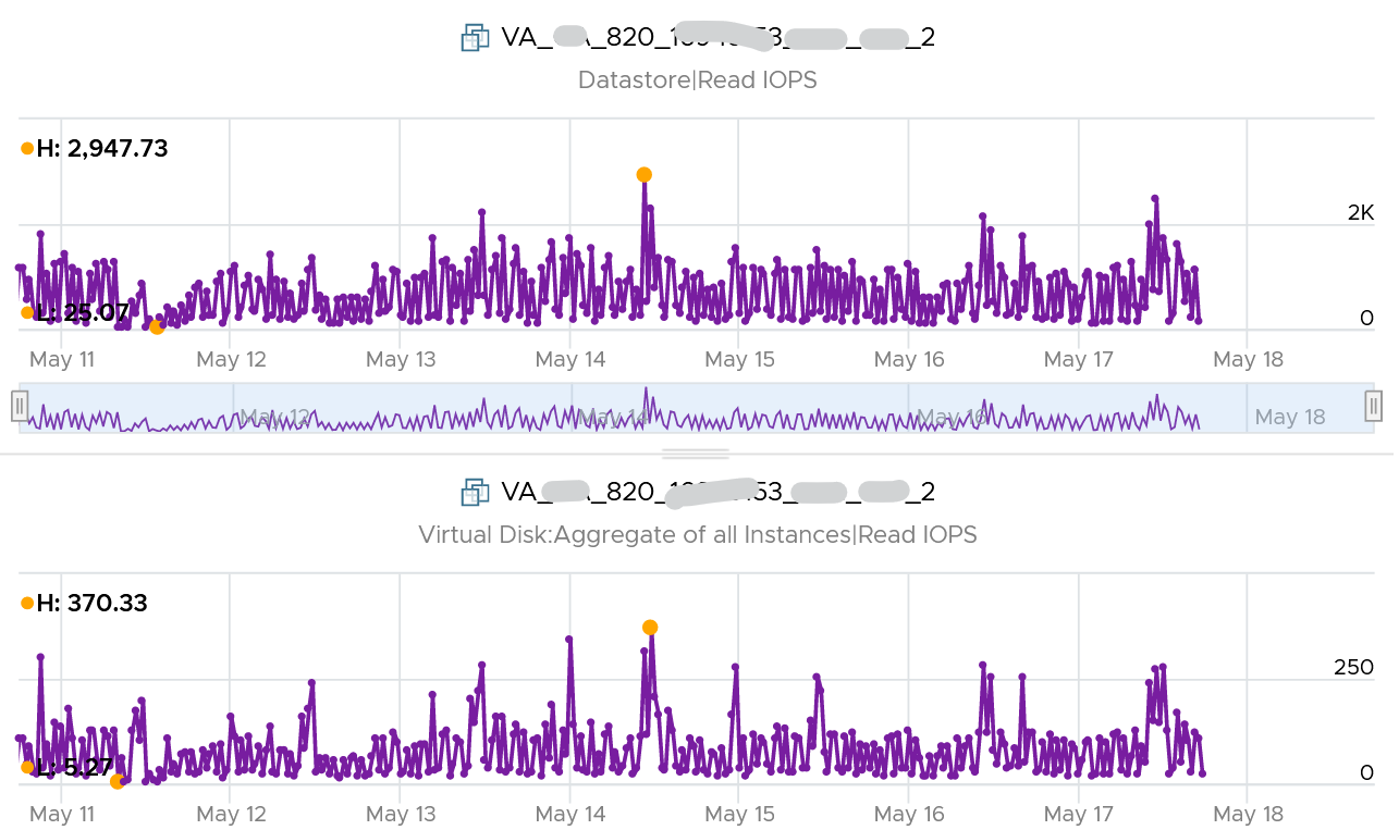
How I know that’s IOPS effect as the throughput is identical. The additional reads do not bring back any data. Using the same VM but at different time period, notice the throughput at both levels are identical.

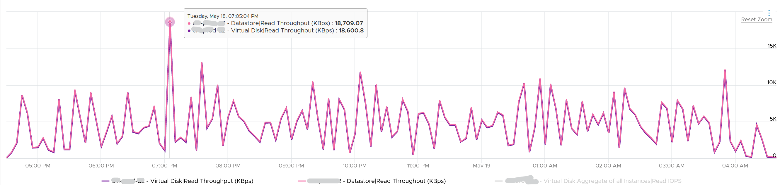
And here is the IOPS on the same time period. Notice the value at datastore layer is consistently higher.

For further reading, Sreekanth Setty has shared best practice here.

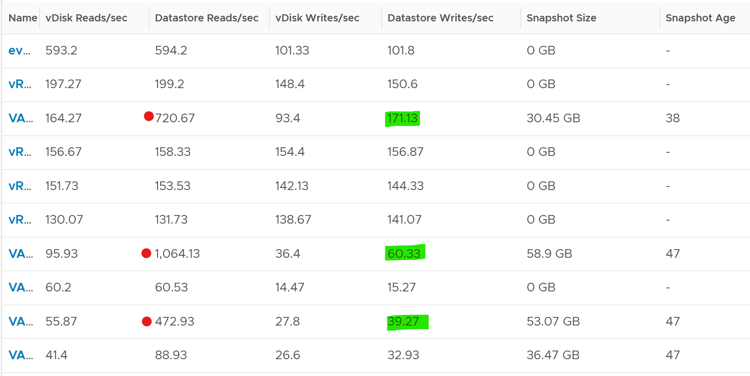
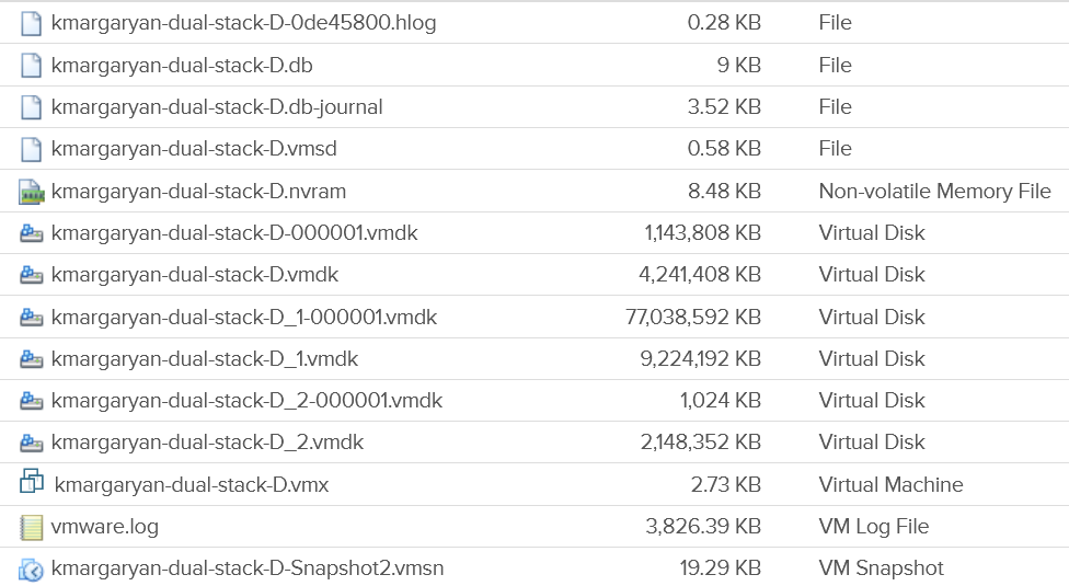
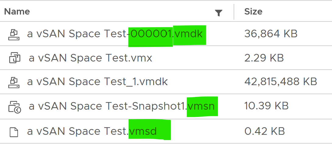
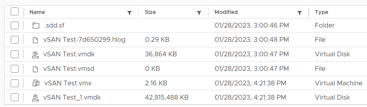
In addition of latency and IOPS, snapshot can also consume more than the actual space consumed by the virtual disk, especially if you are using thin and you take snapshot early while the disk is basically empty. The following VM has 3 virtual disks, where the snapshot file _1-00001.vmdk is much larger than the corresponding vmdk.

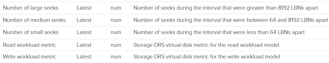
Storage DRS

Lastly, there are storage DRS metric and seek size.

Capacity Metrics

Disk space metrics are complex due the different types of consumption in a single Virtual Disk.

• Actual used by Guest OS

• Unmapped block

• vSAN protection (FTT)

• vSAN savings (dedupe and compressed).

Let’s break it down, starting with understanding the files that make up a VM.

VM Files

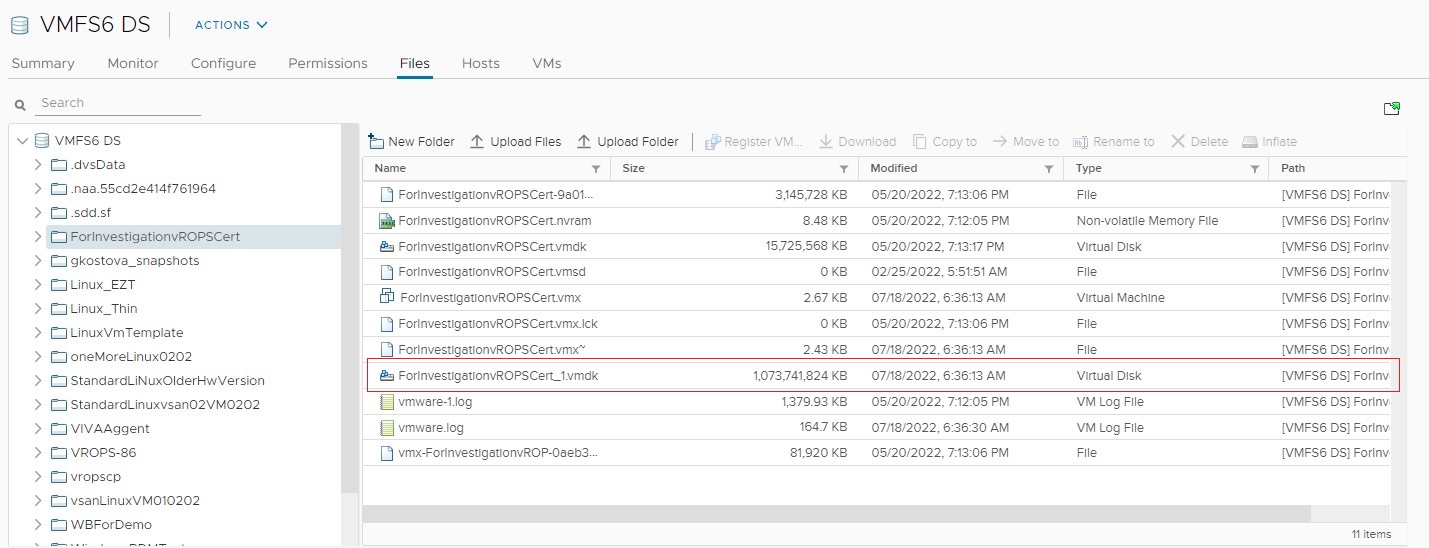
At the end of the day, all those disk space appear as files in the VMFS filesystem, including the RDM pointer files. You can see them when you browse the datastore. The following is a typical example of what vSphere Client will show.

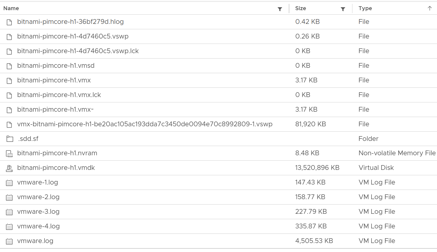
Yes, a lot of files 😊

We can categorize them into 4 from operations viewpoint:

Disk	Virtual disk or RDM. This is typically the largest component. This can be thin provisioned, in which case the provisioned size tends to be larger than the actual consumption as Guest filesystem typically does not fill 100%. All virtual disks are made up of two files, a large data file equal to the size of the virtual disk and a small text disk descriptor file which describes the size and geometry of the virtual disk file. The descriptor file also contains a pointer to the large data file as well as information on the virtual disks drive sectors, heads, cylinders and disk adapter type. In most cases these files will have the same name as the data file that it is associated with (i.e. MyVM1.vmdk and MyVM1-flat.vmdk). A VM can have up to 64 disks from multiple datastores.
Snapshot	Snapshot protects 3 things: VMDK Memory Configuration For VMDK, the snapshot filename uses the syntax MyVM-000001.vmdk where MyVM is the name of the VM and the six-digit number 000001 is just a sequential number. There is 1 file for each VMDK. Snapshot does not apply to RDM. You do that at storage subsystem instead, transparent to ESXi. If you take snapshot with memory, it creates a .vmem file to store the actual image. The .vmsn file stores the configuration of the VM. The .vmsd file is a small file, less than 1 KB. It stores metadata about each snapshot that is active on a VM. This text file is initially 0 bytes in size until a snapshot is created and is updated with information every time snapshots are created or deleted. Only 1 file exists regardless of the number of snapshots running as they all update this single file. This is why your IO goes up.
Swap	The memory swap file (.vswp). A VM with 64 GB of RAM will generate a 64 GB swap file (minus the size of memory reservation) which will be used when ESXi needs to swap the VM memory into disk. The file gets deleted when the VM is powered off. You can choose to store this locally on the ESXi Host. That would save space on vSAN. The catch is vMotion as the swap file must be transferred too. There is also a smaller file (in MB) storing the VMX process swap file. But I’m unsure about this and have not seen it yet.
Others	All other files. They are mostly small, in KB or MB. So if this counter is large, you’ve got unneeded files inside the VM directory. Logs files, configuration files, and BIOS/EFI configuration file (.nvram) Note that this includes any other files you put in the VM directory. So if you put a huge ISO image or any file, it gets counted.

Single VMDK

Let’s review with a single virtual VMDK disk. In the following diagram, vDisk 2 is a thin provisioned VMDK file. It still has uncommitted space as it’s not yet fully used up.

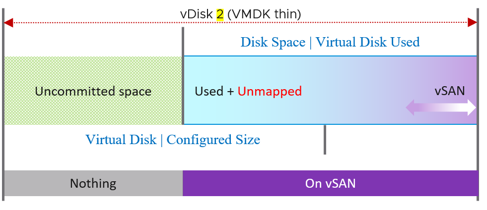
Because vSAN is a software-defined storage, the storage-layer gets mixed up. What operational complexity do you spot from the above diagrams?

• Your unmapped file is also protected by vSAN.

• The uncommitted part does not include vSAN, as it’s yet written.

• You can see that the 2 metrics are not aware of vSAN. vSAN protection (Failure To Tolerate) is shown in purple.

There are 2 metric, shown in Times New Roman font:

Metric	Description
Disk Space | Virtual Disk Used (GB)	The actual consumed size of the VMDK files. It excludes other files such as snapshot files. Note: For RDM the used space is the configured size of the RDM, unless the LUN is thin provisioned by the physical storage array. So its disk space consumption at VM level works like a thick provisioned disk. If this is higher than Guest OS used, and you’re using thin provisioned, then run unmap to trim the unmapped blocks.
Virtual Disk | Configured Size	This metric does not include the vSAN part as it’s taken from consumer layer.

All VM Files

Let’s take an example of a VM with 3 virtual disks, so we can cover all the combinations.

• Thin provisioned

• Thick provisioned

• RDM. Physical or virtual is not relevant.

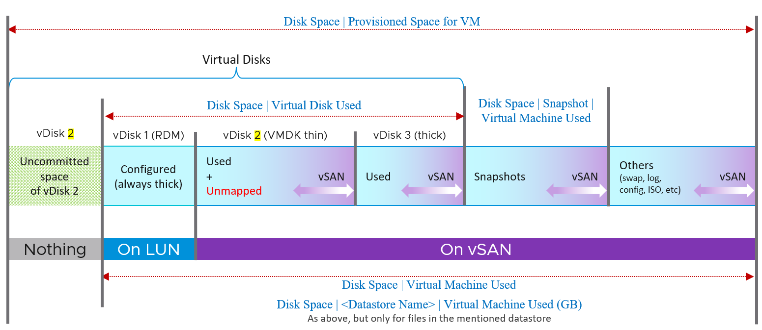
The boxes with blue line show the actual consumption at VM layer. Let’s go through each rectangle.

RDM	It’s not on vSAN as RDM can’t be on a VMFS datastore. It’s mapped to a LUN backed by an external storage. It’s always thick provisioned, regardless of what Windows or Linux uses. The LUN itself could be thin provisioned but that’s another issue and transparent to ESXi (hence VM).
Thin VMDK	We blended vSAN protection into a single box as you can't see the breakdown. It's inside the same file (so there is only 1 file but inside there is actual data + vSAN protection - vSAN dedupe - vSAN compressed). Thin Provisioned can accumulate unmapped block over time. You should reclaim them by running a trim operation. Uncommitted space is the remaining amount that the VMDK can grow into. Since it’s not yet written, it does not have vSAN overhead yet.
Thick VMDK	The Used size equals the configured size as it’s fully provisioned regardless of usage by Guest OS. I’m not sure the final outcome of dedupe and compression. If the Guest OS has not written to it, then I expect the saving will be near 100% in both lazy zero and eager zero.

vSAN protection applies to every file in the datastore. Yes, even your snapshot and log files are protected by default.

All the metrics are under Disk Space metric group. The key ones are:

Metric	Description
Disk Space | Provisioned Space for VM	Just like the Disk Space | Virtual Machine Used (GB), but thin provisioned is based on configured not actual usage. So this metric will have higher value if the thin provisioned is not fully used. This metric is useful at the datastore level. When you overcommit the space and want to know what the total space would be when all the VMs grow to the full size. This metric is not useful for capacity as it mixes both allocation and utilization. BTW, there can be case where the number here is reported as much higher number. See KB 83990. This is fixed in 7.0.2 P03 or 7.0 U2c, specifically in PR 2725886.
Disk Space | Virtual Machine Used (GB)	Just like above, but includes files other than virtual disks. So this metric is always larger. The actual consumed size of the VM files + the configured size of the RDM files. It includes all files in the VM folder in the datastore(s). Formula: Sum ( [layoutEx.file] uniqueSize != null ? uniqueSize : size) / (1024 * 1024 * 1024)
Disk Space | <Datastore Name> | Virtual Machine Used (GB)	Just like above, but only includes files in that specific datastore only. For VM that only resides in 1 datastore, the value will be identical to above.

Snapshot

Disk Space | Snapshot | Virtual Machine Used (GB)

Disk Space used by all files created by snapshot (vmdk and non vmdk). This is the total space that can be reclaimed if the snapshot is removed. Use this to quickly determine which VMs have large snapshot. Formula: Sum of all files size / (1024 * 1024 * 1024)  where aggregation is only done for snapshot files. A file is a snapshot file if its layoutEx file type equals to snapshotData, or snapshotList or snapshotMemory

Disk Space | Snapshot | Access Time (ms)

The date and timestamp the snapshot was taken. Note you need to format this.

vSphere Client UI

I’m adding this just in case you got curious 😊

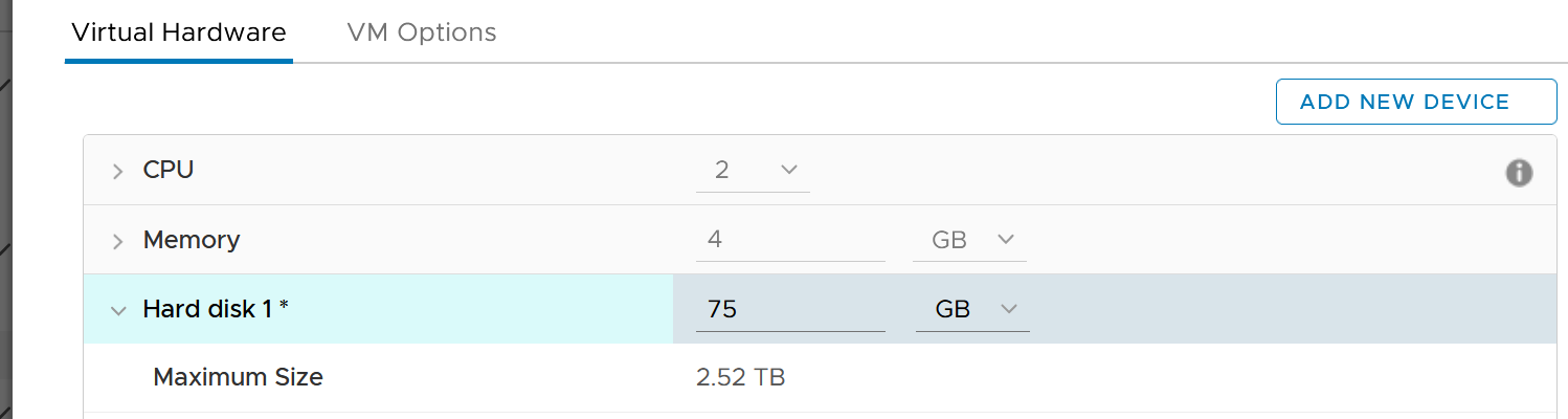
Let’s start with the basic and progress quickly. In the following example, I would create a small VM from scratch, with 2 VMDK disk.

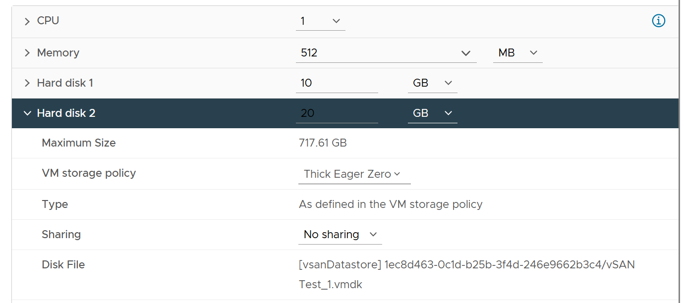
Hard disk 1 is 10 GB. Thin Provisioned. On vSAN.

The VM is powered off. All other settings follow default setting.

I created the VM with just the first disk, to validate the metrics value that will be shown upon creation. What do you expect to see on the vCenter UI?

Here is what I got on vSphere 7.

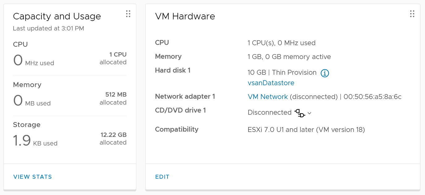
You get 2 numbers, used and allocated, as shown in the Capacity and Usage section.

Used is only 1.9 KB. This is expected as it’s thin provision and the VM is powered off. This is very low, so let’s check the next number….

Allocated is 12.22 GB. This is 10 GB configured + 2.22 GB used. The hard disk 1 size shows 10 GB not 20 GB. This is what is being configured, and what Guest OS see. It is not impacted by vSAN as it’s not utilization.

So you have 2 different numbers for the use portion: 1.9 KB and 2.22 GB.

Why 2 different values?

Let’s see what the files are. We can do this by browsing the datastore and find the VM folder.

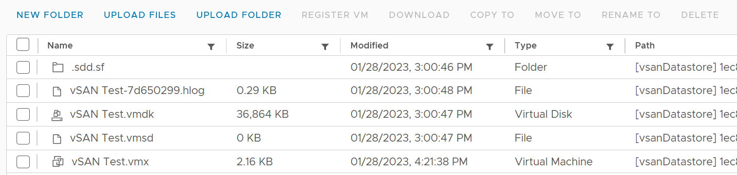
The total from the files above is 36 MB. This does not explain 1.9 KB nor 2.22 GB.

Let’s continue the validation. This time I added Hard disk 2 and configure it with 20 GB. Unlike the first disk, this is Thick Provisioned so we can see the impact. It is also on vSAN.

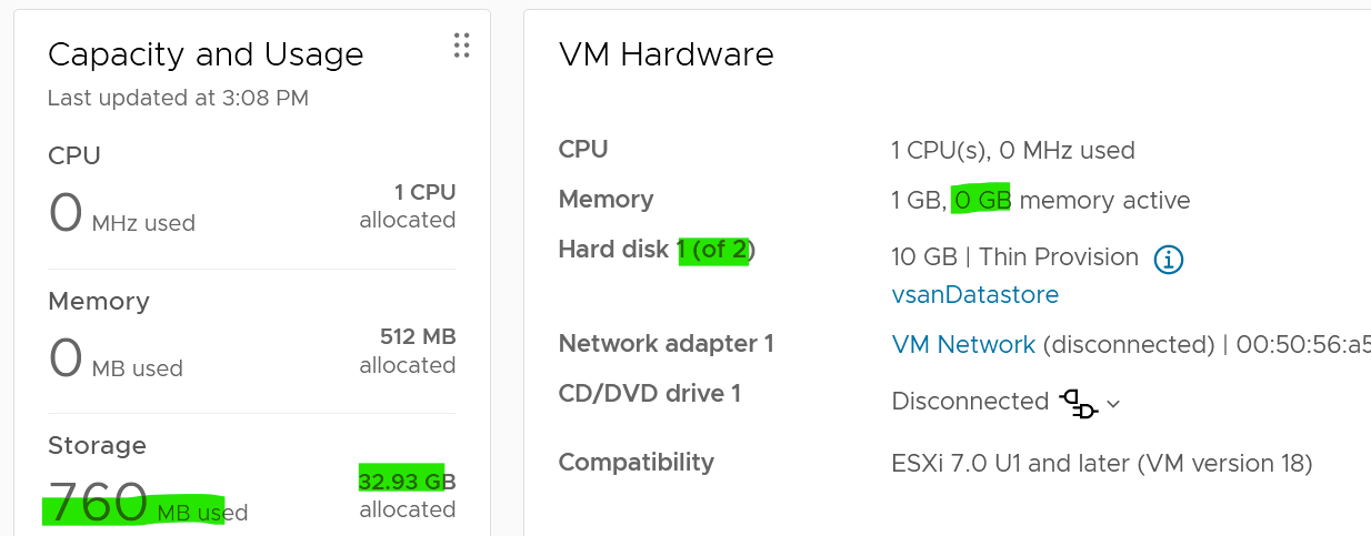
Used has gone up from 1.9 KB to 760 MB. As this is on vSAN, it consists of 380 MB of vSphere + 380 MB of vSAN protection. The vSAN has no dedupe nor compression, so it’s a simple 2x.

Allocated is 32.93 GB as it consists of 30 GB configured and 2.93 GB. This 2.93 is half vSphere overhead + vSAN protection on the overhead.

Looking at the datastore level, the second hard disk is showing 40.86 GB. It maps to hard disk 2.

From this simple example, you can see that Allocated in vCenter UI actually contains used and allocated. By allocated it means the future potential used, which is up to the hard disk configured size. The used portion contains vSAN consumption if it’s on vSAN, while the unused portion does not (obviously since vSAN has not written any block).

ESXi

The following screenshot shows the ESXi metric groups for storage in the vCenter performance chart.

As expected, there are 4 metrics groups for storage

• Datastore

• Disk

• Storage adapter

• Storage path.

We’ve covered earlier how they work together. We also covered how vSAN impacts them.

Disk or Device

There are 3 layers from VM to physical LUN

• VM.

• The kernel. This is measured by the KAVG counter and QAVG counter.

• Device.

Compared with Adapter or Path, you get a lot more metrics for disk or device as there is capacity metric.

As expected, there is no breakdown as the kernel cannot actually see anything in between the HBA and the device. So no metrics such as number of hops as it’s not even aware of the fabric topology.

Contention Metrics

Frank Denneman, whose blog and book are great references, shows the relationship among the counters using the following diagram:

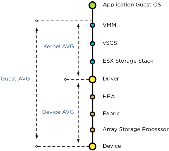
For further reading, review this explanation by Frank, as that’s where I got the preceding diagram from.

Guest Average	GAVG	Guest here means VM, not Guest OS as the counter starts from VMM layer not Windows or Linux.
Kernel Average	KAVG	ESXi is good in optimizing the IO, so in a healthy environment, the value should be within 0.5 ms. This is computed from Guest AVG and Device AVG, which are raw counters.
	QAVG	QAVG, which is queue in the kernel, is part of KAVG. If QAVG is high, check the queue depths at each level of the storage stack. Cody explains why QAVG can be higher than KAVG here. In short, QAVG measures both VM IO and the kernel IO, while KAVG only includes VM IO.
Device Average	DAVG	The average time from ESXi physical card to the array and back. Typically, there is a storage fabric in the middle. The array typically starts with its frontend ports, then CPU, then cache, backend ports, and physical spindles. So if DAVG is high, it could be the fabric or the array. If the array is reporting low value, then it’s the fabric of the HBA configuration. I’m unsure what DAVG measures when it’s vSAN and the data happens to be local.

For each of the above 4 sets, you expect read latency, write latency and the combined latency. That means 12 counters and here are what they are called in vSphere Client UI:

Device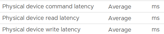
Kernel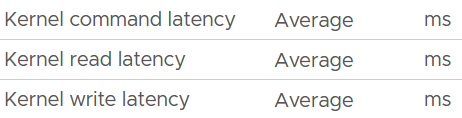
Queue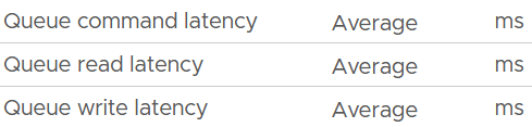
Guest	The counters are not prefixed with Guest, so they are simply called: Command Latency Write Latency Ready Latency

With the above understanding, let’s validate with real world values.

I chose the last ESXi since that’s the one with worst latency.

I plotted Kernel vs Device.

What do you notice? Can you determine which is which?

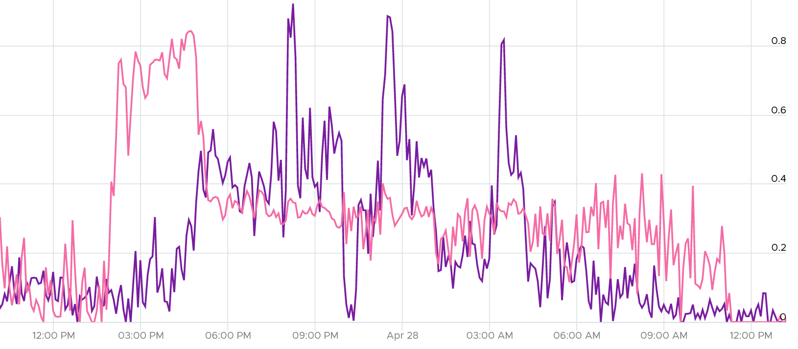
They don’t correlate. This is expected since both have reasonably good value (my expectation is below 0.5 ms).

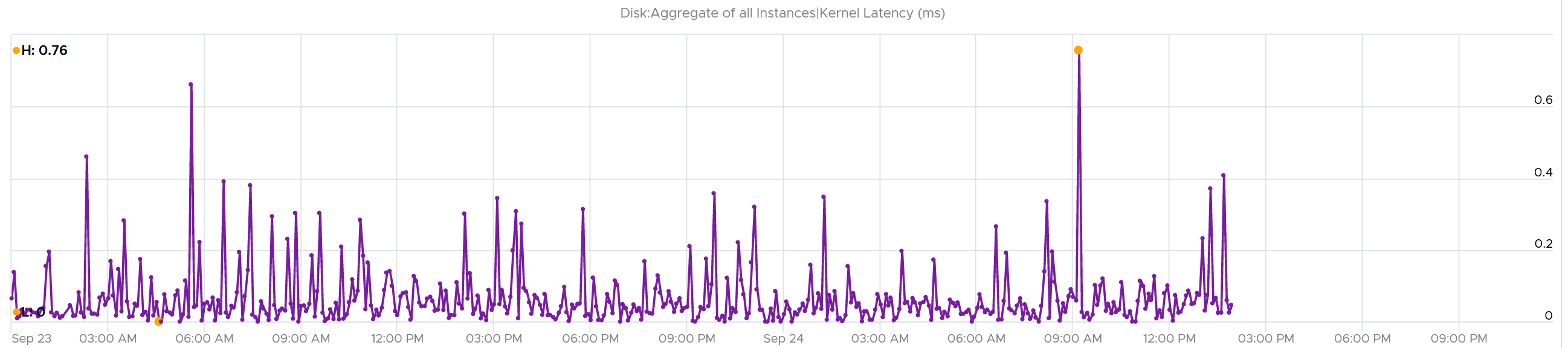
The bulk of the latency should come from the Device. In a healthy environment, it should be well within 5 ms. With SSD, it should be even lower. As you can see below, it’s below 1.75 ms. Notice the kernel latency is 0.2 ms at all times except in 1 spike.

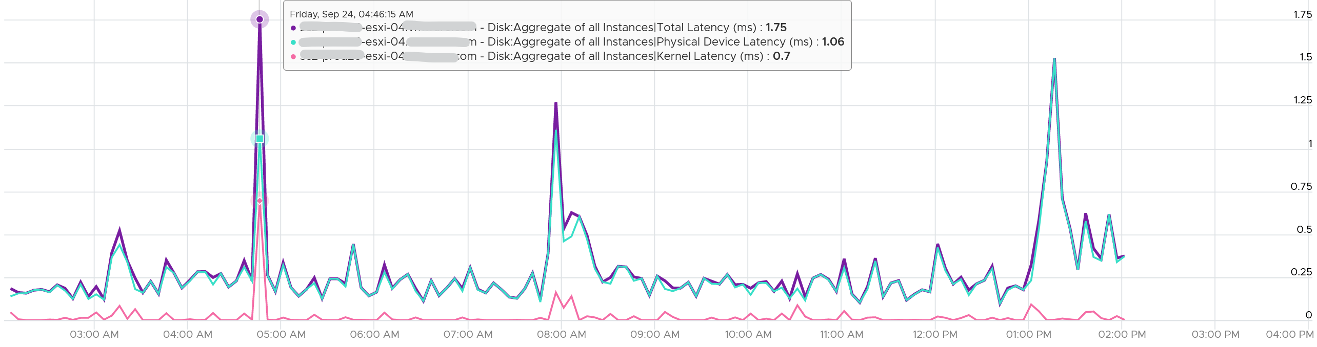
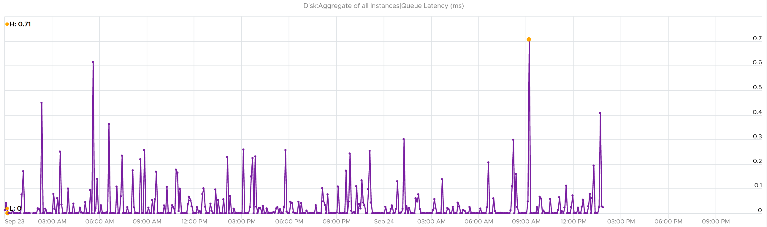
What about the Queue latency? It’s part of the kernel latency, so it will be 100% within it. When the kernel latency value is in the healthy range, the 2 values should correlate, as the value is largely dominated by the Queue. Notice the pattern below is basically identical.

Other Metrics

I find the value of Bus Resets and Commands Aborted are always 0

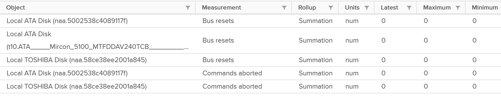
If you’ve seen a non zero let me know.

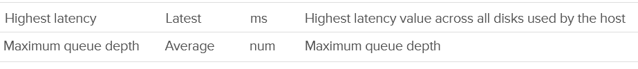
I’m not sure what highest latency refers to (Guest, Kernel, or Device).

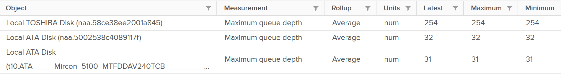
Maximum Queue Depth is more of a property than a metric, as it’s a setting.

Consumption Metrics

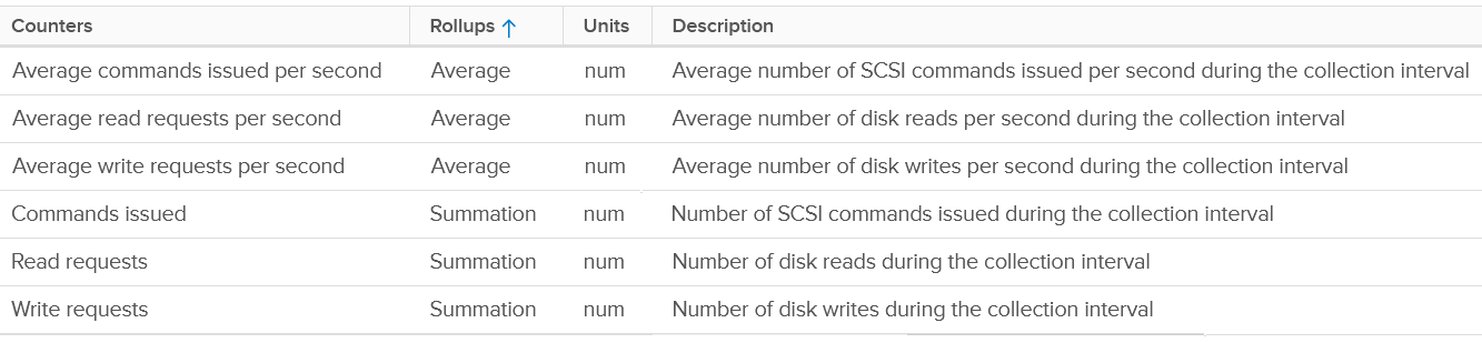
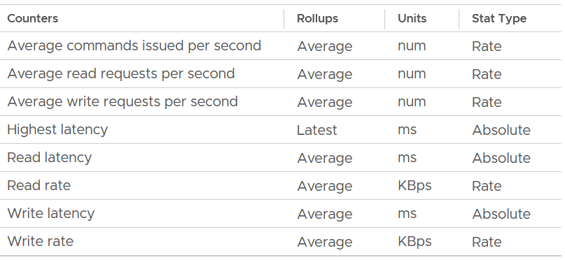
You get the standard IOPS and Throughput metrics.

IOPS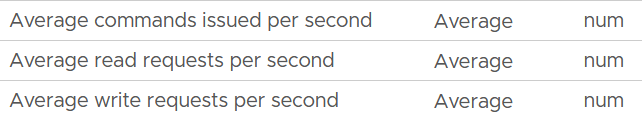
Throughput	The counters names are Read Rate Write Rate Usage All their units are in KB/s
Total IO	This is just the number of Read or Write in the time interval. The counters names are Read Requests Write Requests Commands Issued

Storage Adapter & Path

They have identical set of counters, hence I’m documenting them together. Ideally, adapter should include metrics such as adapter queue length and commands aborted.

The following screenshot shows the metrics provided:

For storage path, the counters may appear that they are measuring the device, as the object name is not based on the friendly name.

The object above is the path, not the device.

Contention Metrics

There are 3 metrics provided:

• Read latency

• Write latency

• Highest latency

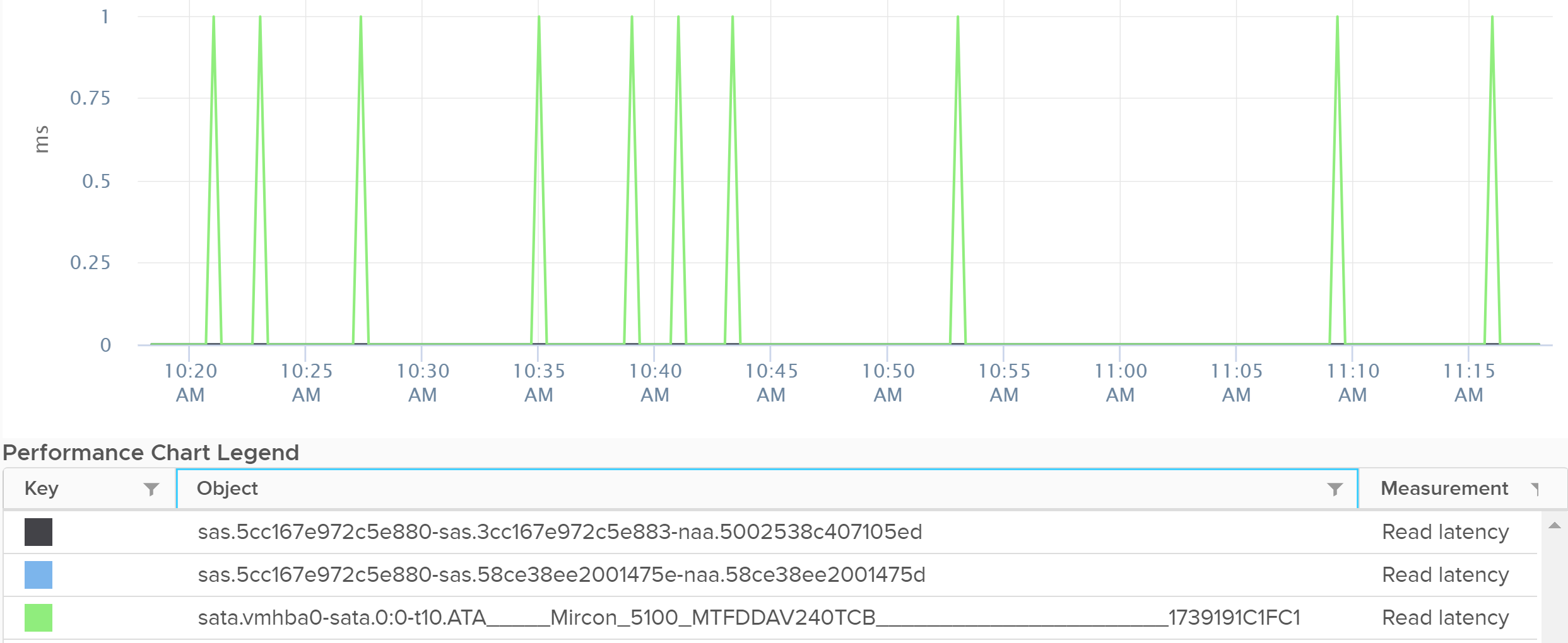
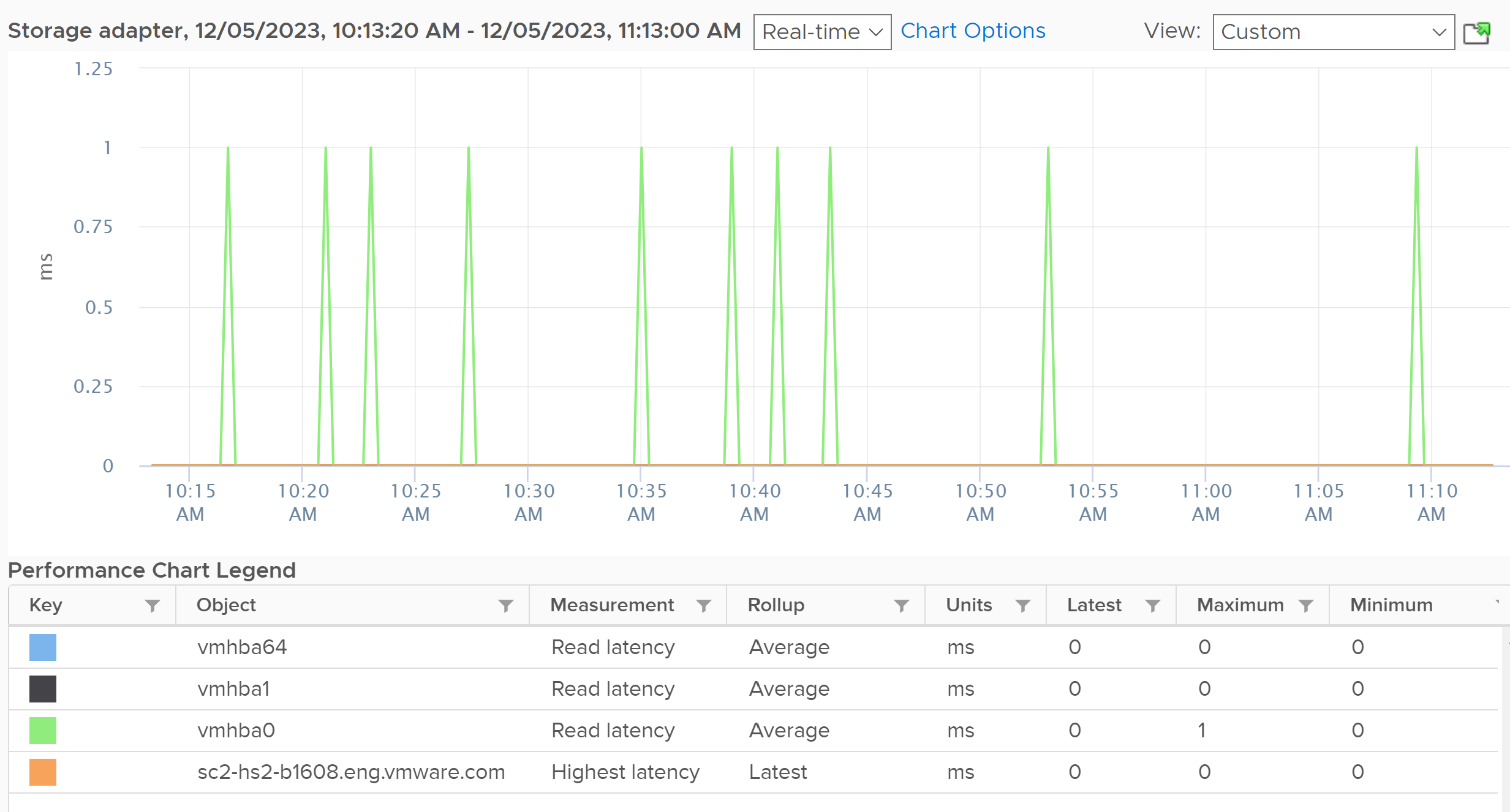
The highest latency metric takes the worst value among all the adapters or the paths. This can be handy compared to tracking each of them one by one. However, it averages each adapter first, so it’s not the highest read or write. You can see from the following screenshot that its value is lower than the read latency or vmhba0. What you want is the highest read or write among all the adapters or paths.

Analysis

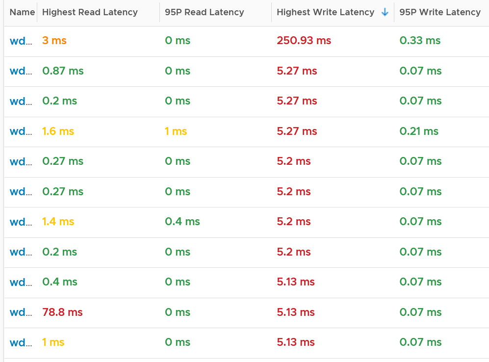
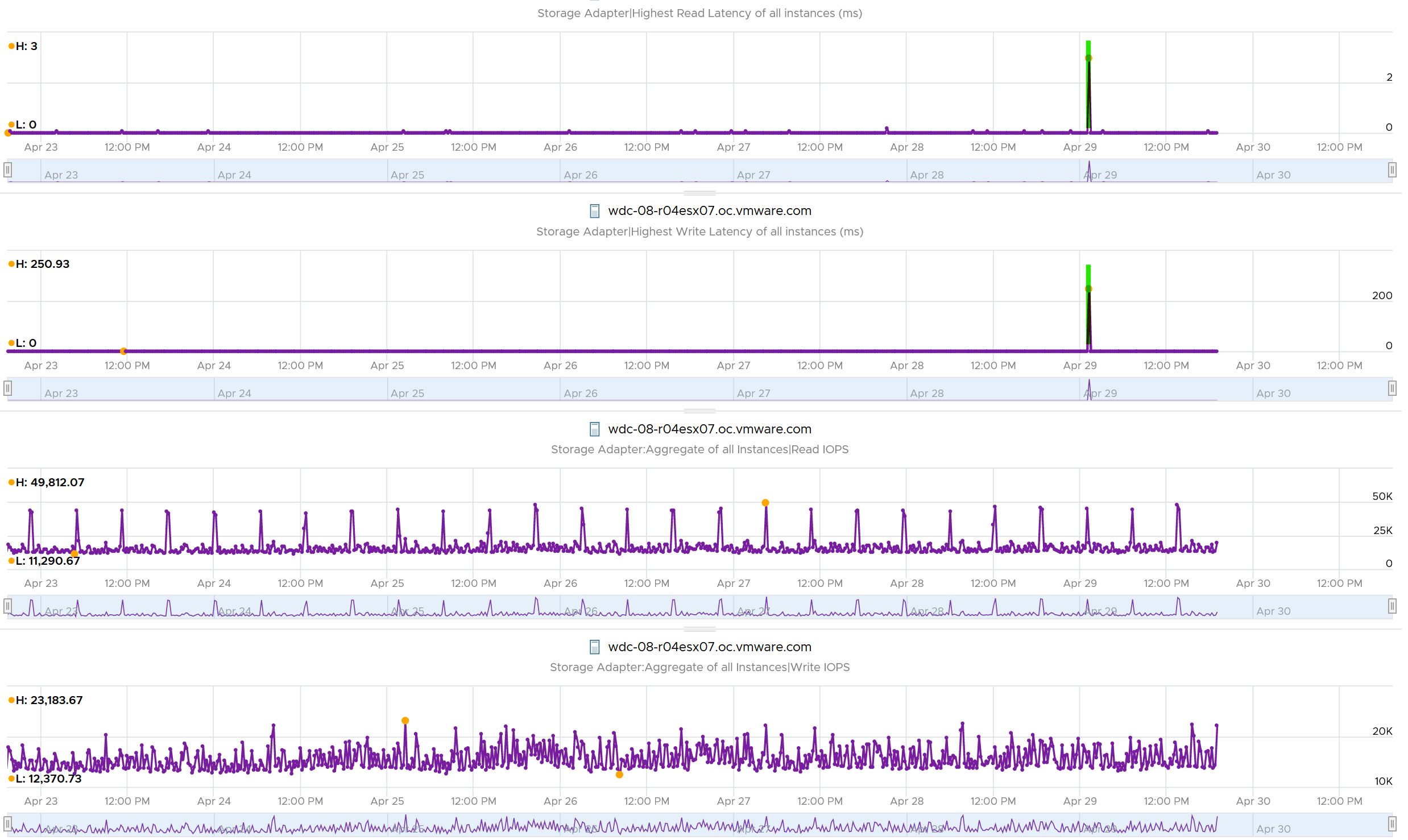
I plotted 192 ESXi host and checked the highest read latency and highest write latency among all their adapters. As the data was returning mostly < 1 ms, I extended to 1 week and took the worst in that entire week. You can see that the absolute worst of write latency was a staggering 250 ms. But plotting the 95^th percentile value shows 0.33 ms, indicating it’s a one off occurrence in that week. The 250 ms is also likely an outlier as the rest of the 191 ESXi shows maximum 5 ms, and with much lower value at 95^th percentile.

Plotting the value of the first ESXi over 7 days confirmed the theory that it’s a one off, likely an outlier.

Does it mean there is no issue with the remaining of the 191 ESXi hosts?

Nope. The values at 95^th percentile is too high for some of them.

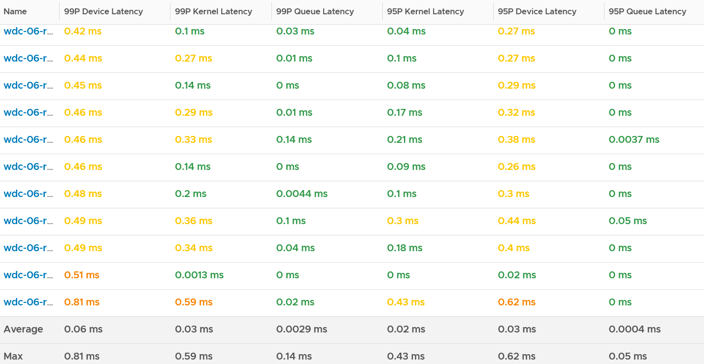
I modified the table by changing Maximum with 99^th percentile to eliminate an outlier. I also reduced the threshold so I can see better. The following table shows the values, sorted by the write latency.

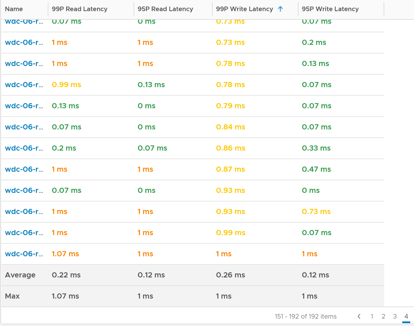
The table revealed that there are indeed latency problem. I plotted one of the ESXi and saw the following.

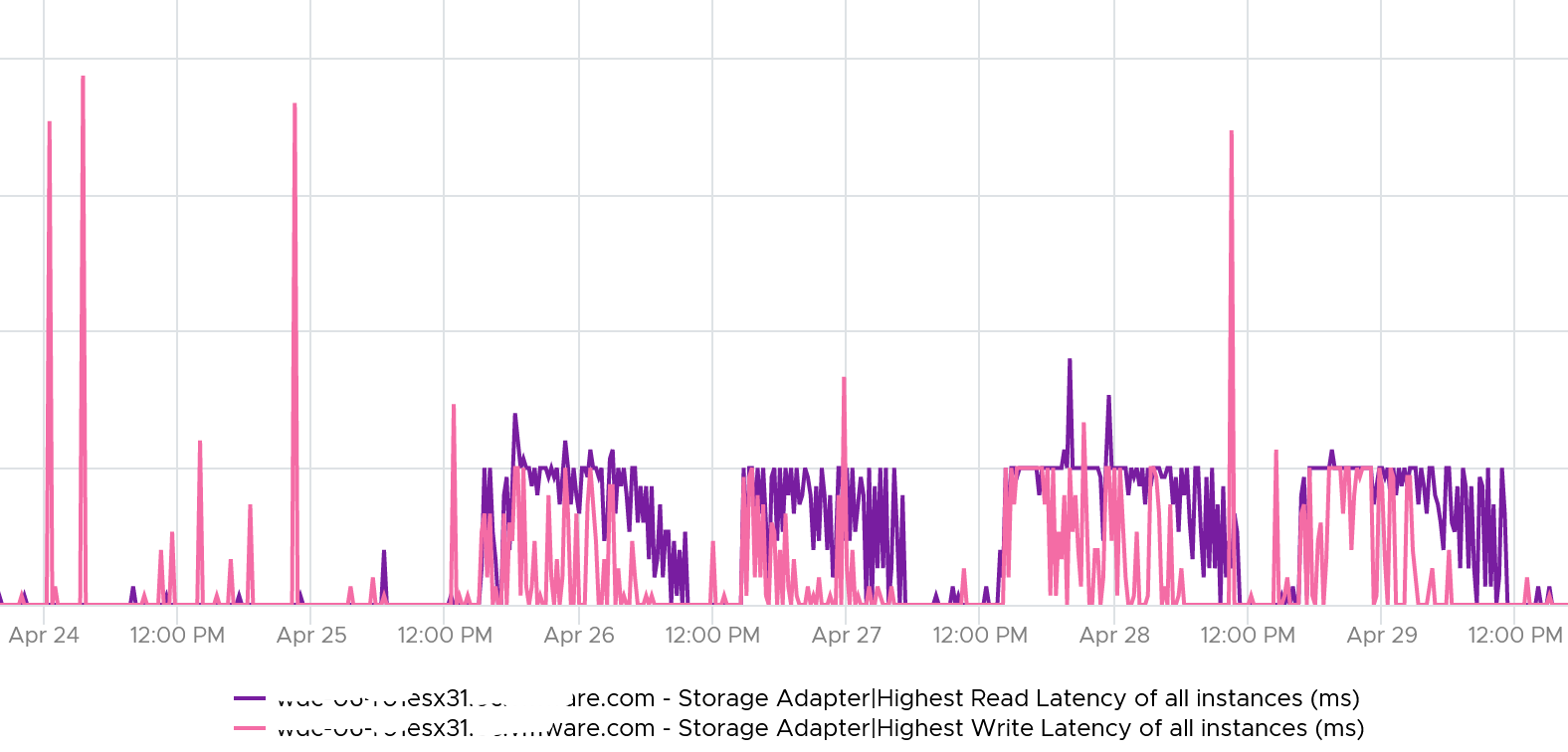
From here, you need to drill down to each adapter to find out which one.

Consumption Metrics

For each adapter, there are 4 metrics provided:

• Read IOPS, tracking the number of reads per second.

• Write IOPS

• Read throughput

• Write throughput.

The following screenshot is an example of what you get from vSphere Client UI.

If the block size matters to you, create a super metric in VCF Operations.

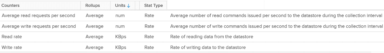
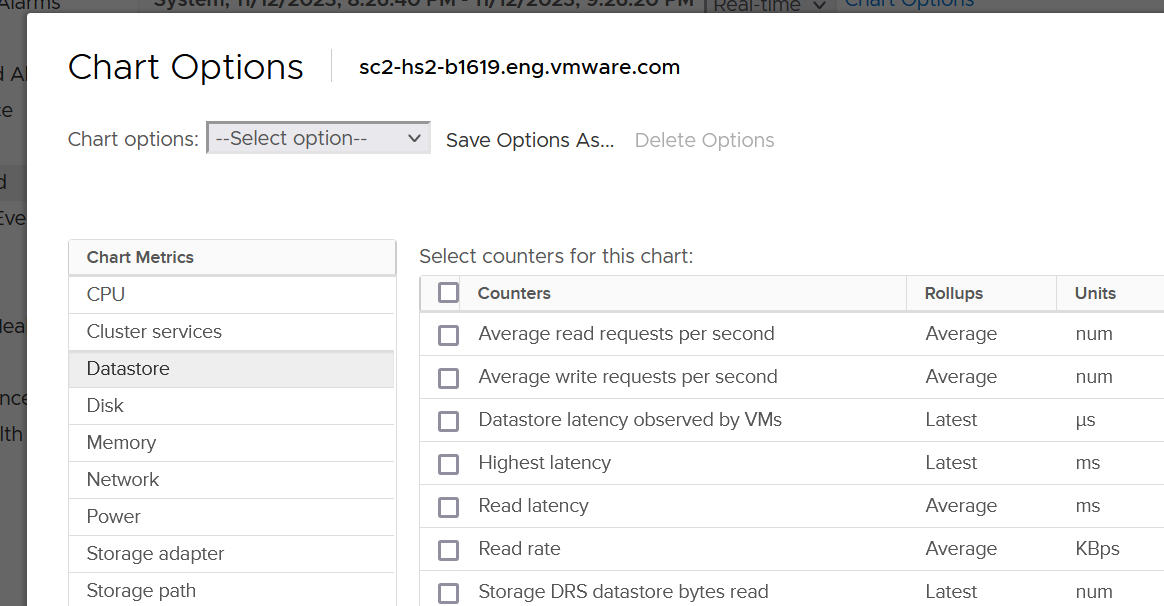
Datastore

For shared datastore, the metrics do not show the same value with the one at datastore object. All these metrics are only reporting from this ESXi viewpoint, not the sum from all ESXi mounting the same datastore. As a result, I’d cover only performance. Capacity will be covered under the datastore chapter.

For each datastore, you get the usual IOPS, throughput and latency. They are split into read and write, so you have 3 x 2 = 6 metrics in total. These are the actual names:

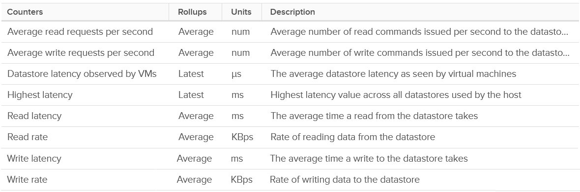
There is no block size but you can derive it by dividing Throughput with IOPS.

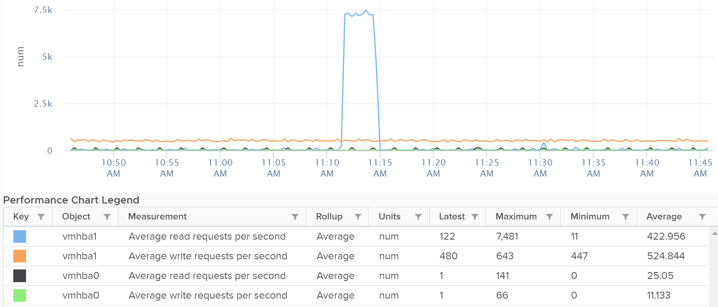
You also get 2 additional counters:

• Datastore latency observed by VMs

• Highest latency.

I plotted their values and to my surprise the metric Datastore latency observed by VMs is much higher. You can see the blue line below. It makes me wonder what the gap is as there is only the kernel in between.

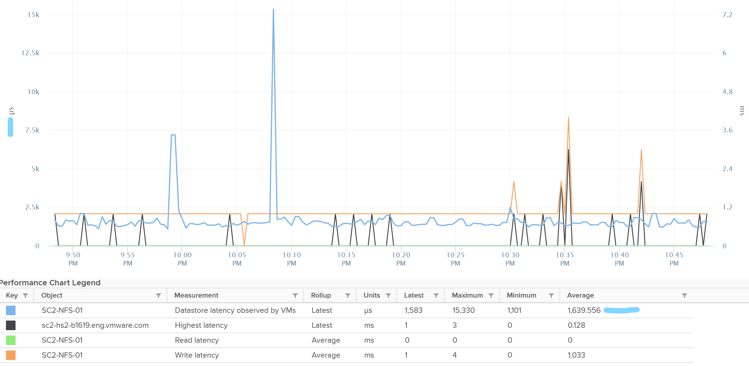
The metric Highest Latency is a normalized averaged of read and write, hence it can be lower.

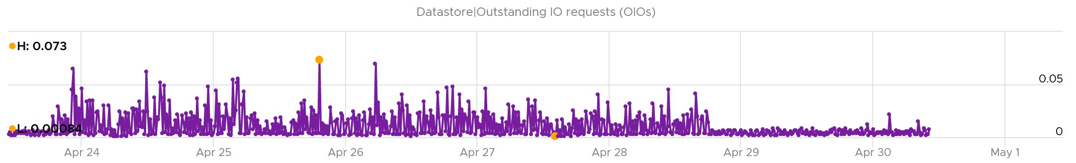
Outstanding IO

You can derive the outstanding IO metric from latency and IOPS. I think latency counter is more insightful. For example, the following screenshot shows hardly any IO being in the queue:

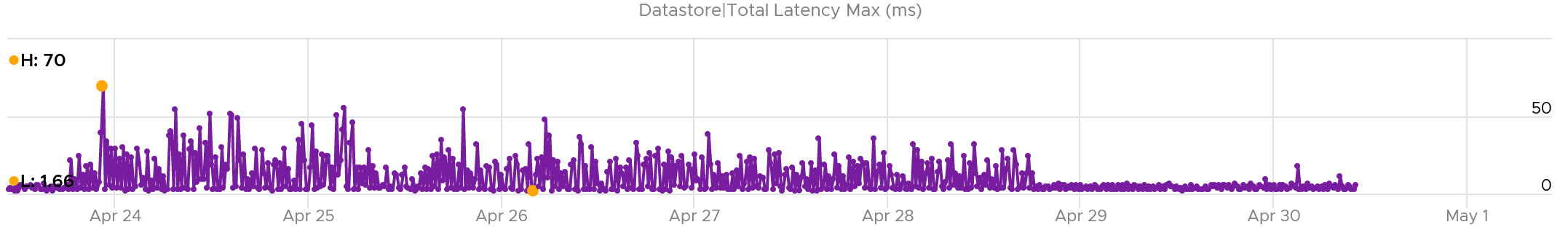
However, if you plot latency, you get same pattern of line chart but with higher value.

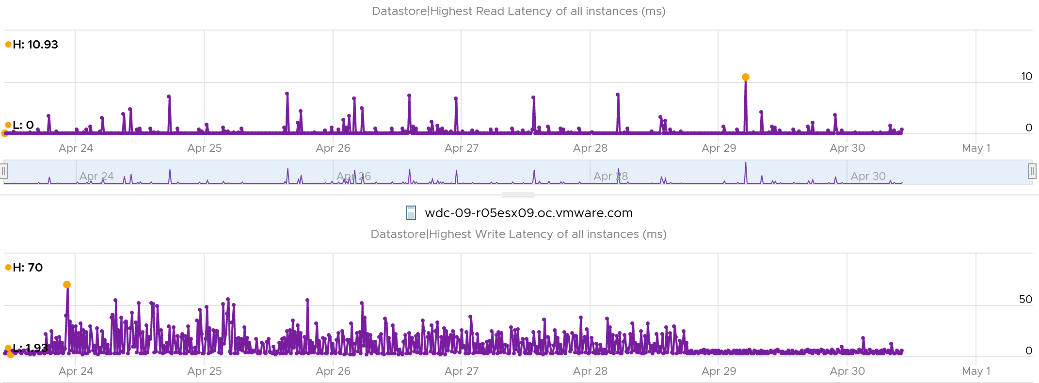
You can check whether it’s read or write by plotting each.

The following screenshot shows it’s caused by write latency. It’s expected if your read is mostly served by cache.

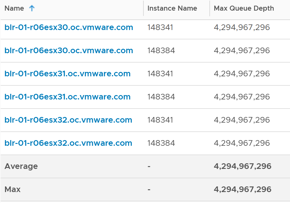
Queue Depth

You can also see the queue depth for each datastores (I think this is actually the backing LUN, but unsure if there are extent). Ensure that the settings are matching your expectation and are consistent. You can list them per cluster and see their values.

Chapter 5